


The following text is based on Boschini et al. (2024) and regards the HelMod-4/CUDA version for GPU architectures (see also Boschini et al. 2023, Della Torre et al. 2023).
As shown here, in HelMod the Parker transport equation is solved numerically by employing the Monte Carlo integration of an equivalent set of stochastic differential equations (SDE). The integration algorithm structure of SDE is very suitable for parallel computing, particularly GPU architectures. This property allows the possibility to design accelerated algorithms and then increase the performances of the computation.
In this field, the use of GPUs for this purpose represents a huge speedup in computing the GCR solar modulation, opening the feasibility of additional studies that need a large number of simulations and the systematical application to the assessment of space radiation effects considering those cases like deep-space missions for which GCRs are largely contributing to hazard. In fact, assessing the GCR contribution to the space radiation environment is a complex operation due to the time variability of GCR flux. Physically motivated models like HelMod-4 are key tools used to describe the transport of particles through the interplanetary medium. These methods have been used up to now only by specialists due to the long computational effort needed. Now, thanks to GPU algorithms like the one presented in this paper, these models will surely become achievable by general-purpose users.
In this section, we present the results of the GPU-accelerated algorithm applied to the HelMod-4 model. In Section 1, it is shown that HelMod-4 and HelMod-4/CUDA can be equivalently used to provide solar-modulated spectra with a similar degree of accuracy in reproducing observed data. In addition, the observed performances of the GPU algorithm represent a huge improvement with respect to the initial HelMod-4 code, quantified as an average improving factor of ~40 in run speed-up for the case of 5000 quasi-particles, as shown in Section 2. A complete description of the GPU implementation can be found in Boschini et al. (2024). In Section 3 the GPU farm at the University of Milano Bicocca is described.
1. Algorithm validation
To validate HelMod-4/CUDA we compared the numerical result with those obtained by HelMod-4 on CPU architecture.
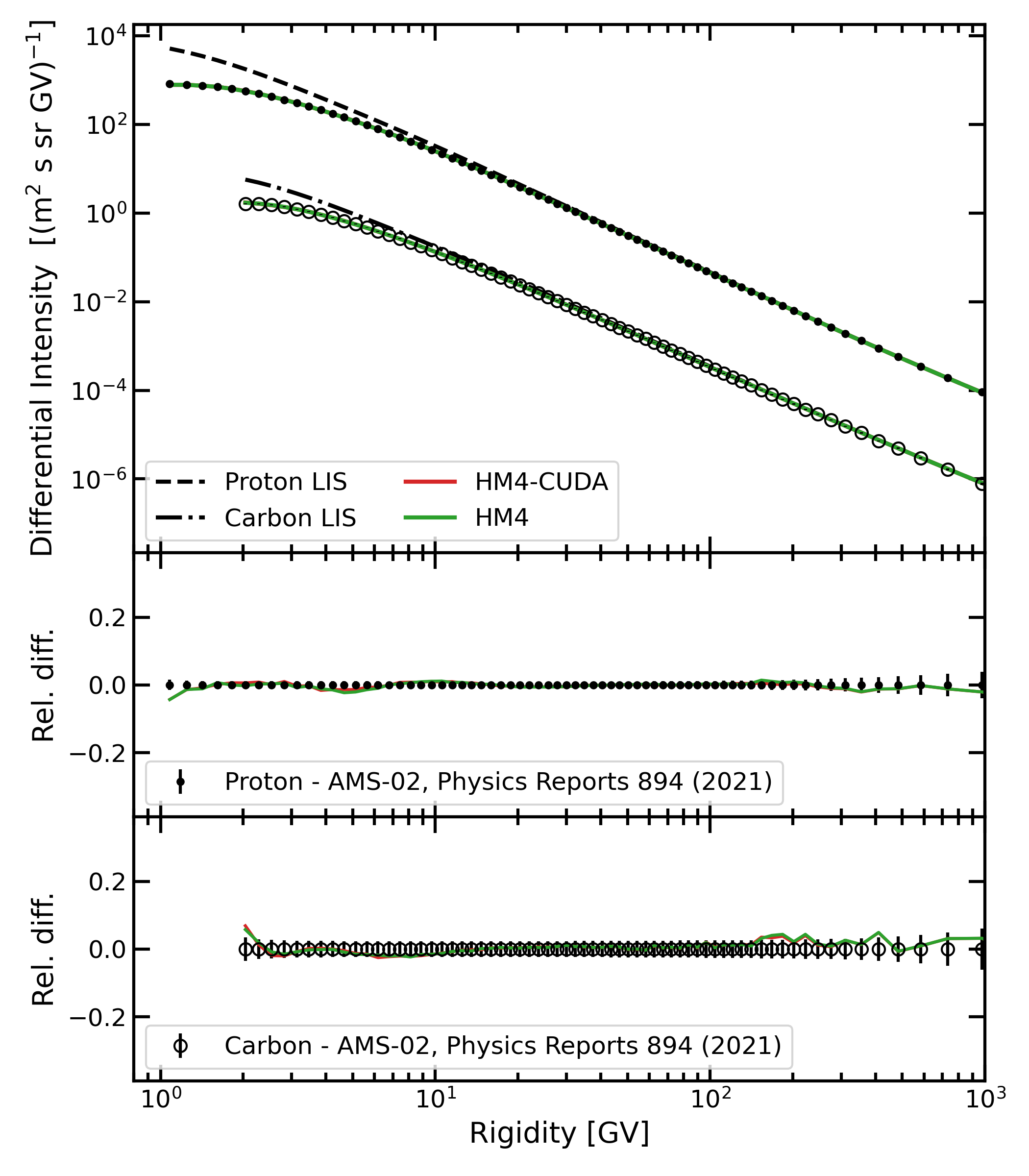
Fig. 1. Top panel: Modulated differential intensity of GCR proton and carbon spectra as obtained from HelMod-4 (green) and HelMod-4/CUDA (red) for the integrated period 2011–2018. Dashed and dot-dashed lines represent, respectively, the proton and the carbon LIS as defined in Boschini et al. (2020b). Black points and empty circles represent, respectively, proton and carbon spectra as measured by AMS-02 and reported in Aguilar et al. (2021). The color code is the same in the other panels of this figure. Middle (Bottom) Panel: Relative difference of HelMod-4 (HM4) and HelMod-4/CUDA (HM4-CUDA) modulated spectra with AMS-02 protons (carbon) observations, whose relative uncertainties are reported in black, for the same time interval. In all panels, red and green curves almost overlapped since the differences between HM4 and HM4-CUDA are below a few percent and experimental uncertainties. [Figure from Boschini et al. (2024)]
In Fig. 1 we show modulated spectra of proton and carbon GCR measured by AMS-02 (Aguilar et al., 2021) along with the differential intensities computed by HelMod-4 (green) and HelMod-4/CUDA (red) for the same period. The second and third panels of Fig. 1 report the relative difference of simulations from experimental data. From this figure, it is hard to distinguish results coming from the two algorithms. Differences are consistent with the uncertainties due to simulated statistics in the Monte Carlo solvers. The same comparison was performed, providing similar results, with all the experimental datasets used to validate the HelMod-4 model within the HelMod-GALPROP framework.
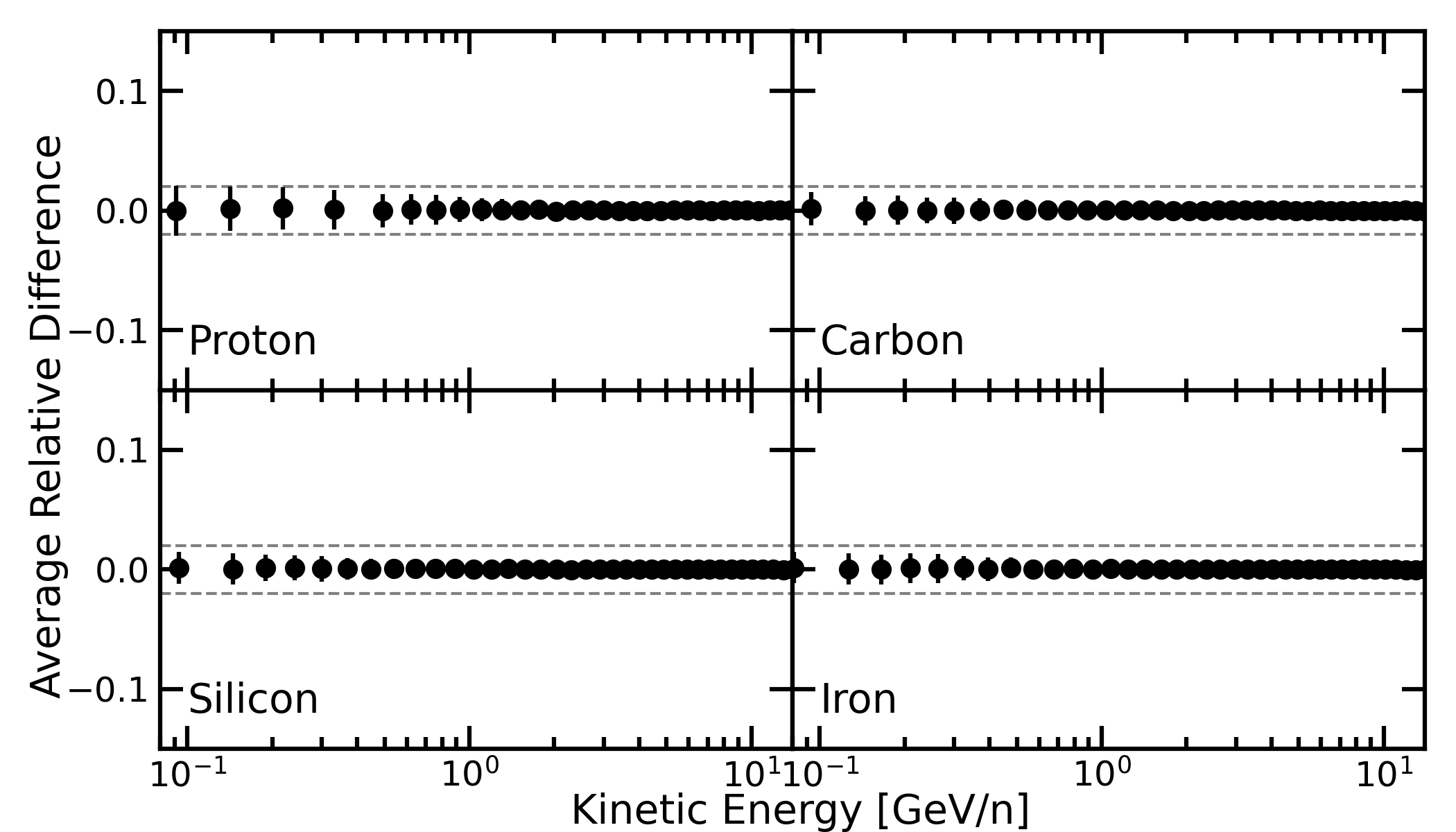
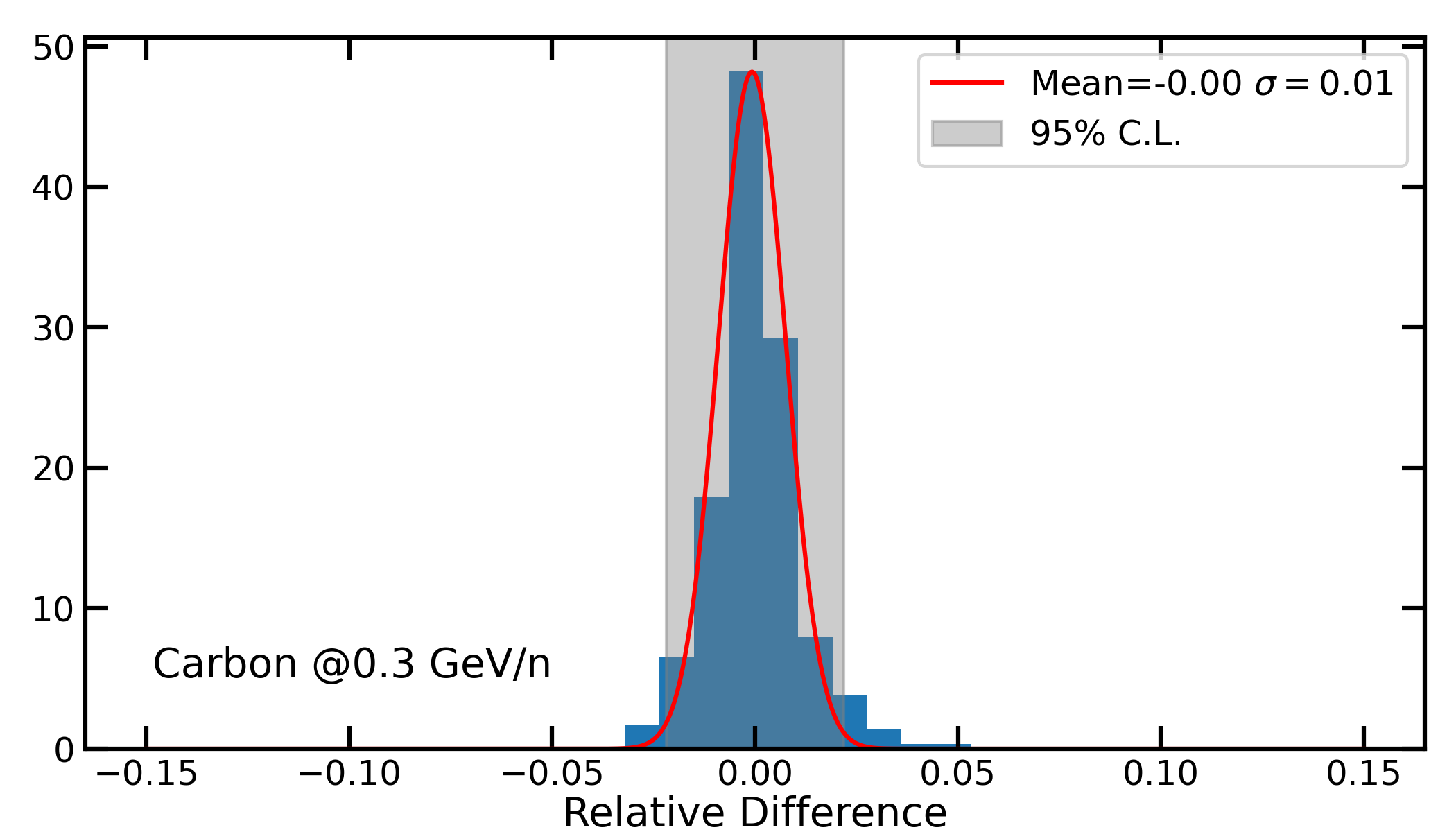
Fig. 4. Relative difference of HelMod-4/CUDA results with respect to the HelMod-4 ones. The left panel summarizes the mean relative differences computed for each bin in the time interval from 2020 to 2046. The values are computed for proton-, carbon-, silicon- and iron-modulated spectra. The horizontal dashed black lines mark the ∼ 2% uncertainty level. The right panel reports an example of how each point in the left panel is computed: for each energy bin we evaluated the distribution of the relative differences of the algorithms in the time interval 2020–2046 for each Carrington rotation. Then, the mean and standard deviation are computed. In this plot, we superimposed a Gaussian fit and the grey band represents the 2-σ uncertainty. [Figure from Boschini et al. (2024)]
For a more general comparison, we considered the period 2020--2046 and the energy range from 0.1 to 20 GeV/n. This period covers a complete solar cycle in both polarities and considers the two typical usages of HelMod-4: reproducing past measurements and forecasting GCR intensities for future space missions (for a discussion on how the forecast is implemented in HelMod-4 see here). Each simulation was compared bin-by-bin to compute the relative difference of HelMod-4/CUDA results with respect to the HelMod-4 ones (see Fig. 2 - left). For each bin, the mean relative difference and the standard deviation were computed. As reported in Fig. 2 - right, representative of a typical result, the relative differences are distributed normally around zero. This means that the new algorithm does not introduce a significant systematic difference from the CPU one.
The results of this comparison, for all energy bins, are summarized in Fig. 2 - left for four of the most abundant GCR species (proton, carbon, silicon, and iron). The fact that the relative difference between the two algorithms is well confined within the 2% bands (horizontal dashed black line) is proof of the equivalence of the Monte Carlo solvers. All the other ions behave similarly. In other words, HelMod-4 and HelMod-4/CUDA can be equivalently used to provide solar-modulated spectra with a similar degree of accuracy in reproducing observed data.
2. Code Performances
The main motivation for developing a GPU-accelerated algorithm is the boost in performance. In this section, we show the performance of HelMod-4/CUDA algorithm with respect to HelMod-4 (i.e. the CPU code version) using the same parameters.
HelMod-4 was executed on a server with two CPU Intel(R) Xeon(R) 2.10GHz. Since the algorithm used by HelMod-4 does not use any software parallelization technique (i.e. each program uses one CPU-core), we recursively execute at the same time 30 \helmodf{} instances in order to not saturate the CPU resources.
HelMod-4/CUDA was executed on the same server with two GPU NVIDIA A30 Although HelMod-4/CUDA was designed to use all GPUs available, for these tests we forced the code to use only one GPU, allowing it to execute at the same time 2 HelMod-4/CUDA instances. Moreover, the code was compiled with the compilation flag --use_fast_math which would result in lower numerical accuracy but with a huge improvement in reducing the run time.
To evaluate the code performances under different working conditions, we computed the execution time of several energy bins and with a different number of quasi-particle objects from N=102 to 105. This measurement is obtained by averaging over ~200 HelMod instances. In this study, we considered 3 different Carrington rotations (i.e. CR numbers CR-1937, CR-2091, and CR-2132) corresponding to two consecutive solar minima (with opposite solar polarity) and a solar maximum period. The results among the three different periods are qualitatively similar, producing the same relative dependence from N but with different absolute normalization due to the different modulation parameters.
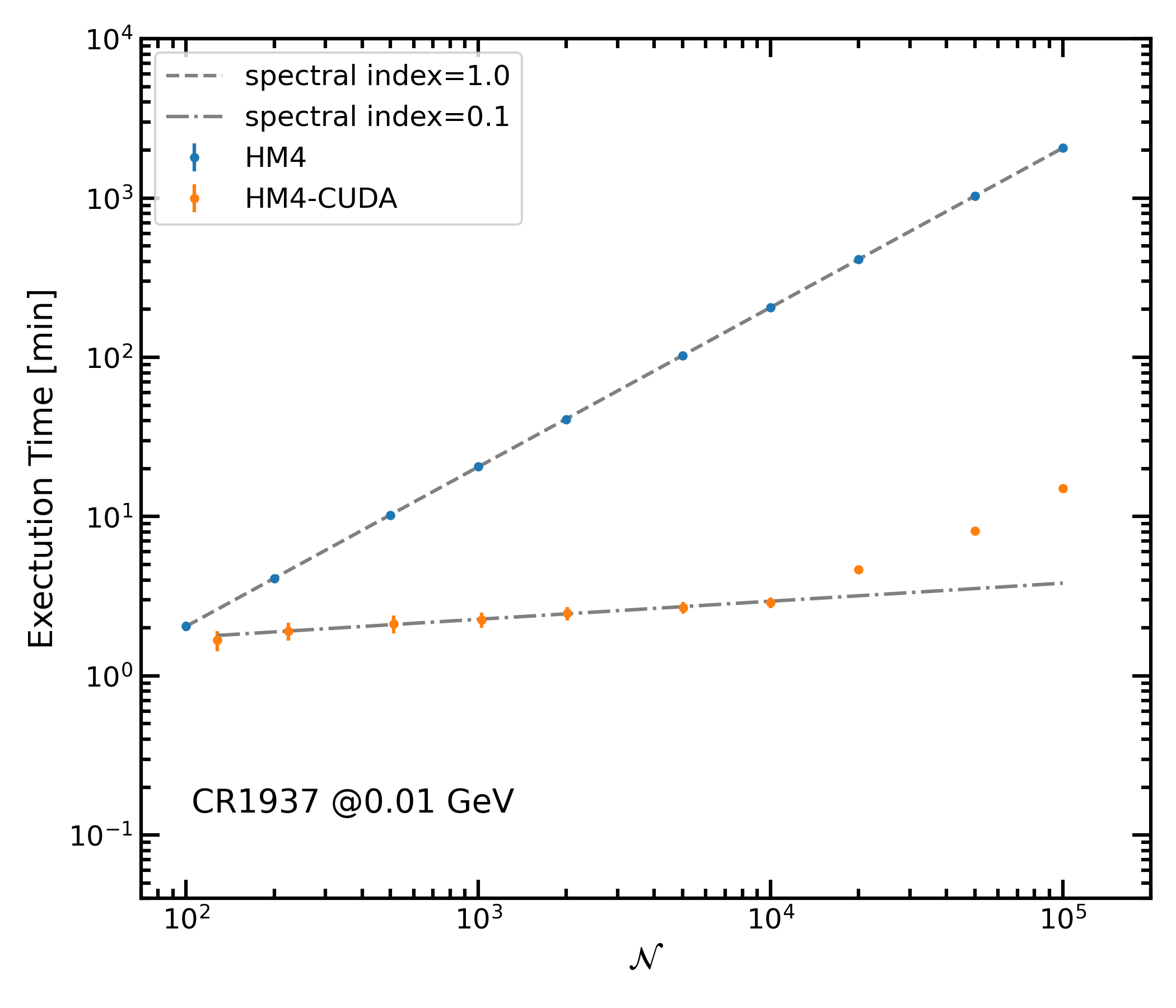
Fig. 3. HelMod-4 (blue points) and HelMod-4/CUDA (orange points) execution time in minutes with respect to the number of simulated events N for the case of 0.01 GeV GCR protons at Earth orbit on CR-1937. The grey lines represent the linear fit of the point in the N-range 102 ∼ 104. HelMod-4/CUDA execution times are evaluated by using 1 GPU board. [Figure from Boschini et al. (2024)]
In Fig. 3 the execution time in minutes of the two algorithms is shown as a function of N. Due to the linearity of the algorithm, the execution time of HelMod-4 scales as a power law of N with spectral index 1, i.e. a linear function. On the other hand, the execution time of HelMod-4/CUDA shows two different regimes: up to N~104 it scales as a power law with spectral index ~0.1, then the spectral index becomes steeper. This is because at N~104 the program saturated the GPU resources and additional operations are required. At N~105 we also register sporadic illegal memory errors. The observed performances represent a huge improvement with respect to the initial HelMod-4 code.
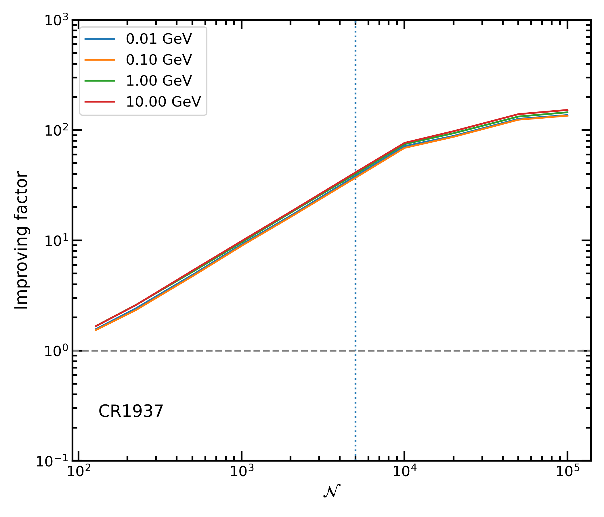
Fig. 4. Improving factor in processing speed by using GPU algorithm with respect to the CPU one. Simulations are performed for GCR protons at Earth orbit on CR-1937 and for four different initial energies. The factor is computed by the ratio of points in Fig. 3 interpolated to match the same N-value. [Figure from Boschini et al. (2024)]
In Fig. 4 we reported the improving speed-up factor evaluated as the ratio between HelMod-4 and HelMod-4/CUDA execution time for proton GCR during the CR-1937 for several kinetic energy. The results for CR-2091 and CR-2132 are similar and confirm an average improving factor of ~40 in run speed-up for the case of N~5000. One has to note that a similar improvement factor could be obtained also by a proper CPU paralleling algorithm, using all the available CPU cores. Anyway, the availability of high-performance GPUs at affordable cost makes the GPU solution very competitive. In addition, the possibility to install several GPUs on a relatively small cluster, if compared with a configuration hosting the same number of CPU cores, makes this solution also much more reliable in terms of requested room, power, and services.
3. GPU Farm
A dedicated ASIF datacenter with 10 NVIDIA GPUs was deployed at the University of Milano-Bicocca, additional GPU cards will be available soon.

Bibliography
Aguilar, M., Ali Cavasonza, L., Ambrosi, G. et al. (2021).Aguilar, M., Ali Cavasonza, L., Ambrosi, G. et al. (2021). The Alpha Magnetic Spectrometer (AMS) on the International Space Station: Part ii – results from the first seven years. Physics Reports, 894, 1 – 116. doi:10.1016/j.823 physrep.2020.09.003.824
Boschini, M., Della Torre, S., Gervasi, M. et al. (2023). Predicting galactic cosmic ray intensities in the heliosphere employing the HelMod model. In Proceedings of 38th International Cosmic Ray Conference —PoS(ICRC2023) (p. 1289). volume 444. doi:10.22323/1.444.1289
Boschini et al (2024), Fast and accurate evaluation of deep-space galactic cosmic ray fluxes with HelMod-4/CUDA, M. J. Boschini, G. Cavallotto, S. Della Torre, M. Gervasi, G. La Vacca, P. G. Rancoita, M. Tacconi, Advances in Space Research, April 2024, In Press
Della Torre, S., Cavallotto, G., Besozzi, D. et al. (2023). Advantages ofGPU-accelerated approach for solving the Parker equation in the heliosphere. In Proceedings of 38th International Cosmic Ray Conference —PoS(ICRC2023) (p. 1290). volume 444. doi:10.22323/1.444.1290.
- Details
- Hits: 5446
At present, the HelMod modulated spectra framework does not include ultra-heavy galactic cosmic ray ions (UHGCRs, i.e., GCRs with Z>28) due to their expected negligible contribution to the radiation risk evaluation (e.g., SEE rate) in space, particularly when compared to the impact of iron (see Appendix A in Boschini et al. 2024).
UHGCRs are GCRs that are heavier than nickel, i.e. with a nuclear charge larger than 28. The origin of UHGCRs is a long-standing and important question in the fields of astronomy and astrophysics (see recent reviews inWiedenbeck et al., 2007; Lingenfelter, 2019; Tatischeff et al., 2021, and references therein). Due to their rarity, measuring their abundance is extremely challenging, and their spectral shape as a function of energy is still unknown. Data mainly consists of ratios of elements or groups of elements in an unspecified energy band. This is due to the limitations of the detectors used to evaluate the abundance, which is typically measured in a range of energies around a few GeV/nucleon.
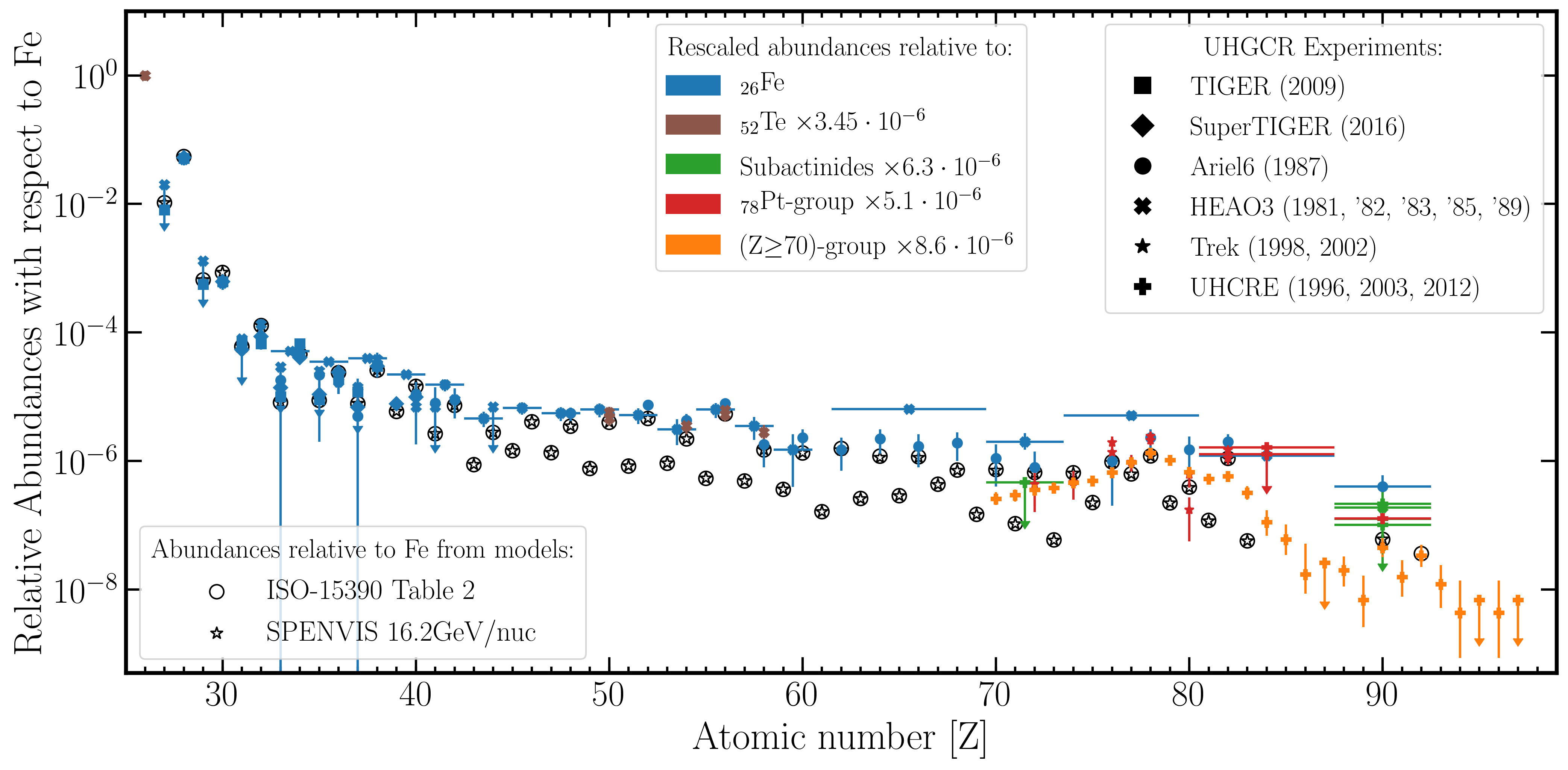
Fig. 1. Relative abundances of GCRs from iron (Z=26) to berkelium (Z=97). Open circles represent GCR relative abundances taken from Table 2 of the ISO-15390 model (ISO, 2004). SPENVIS spectra at 16.2 GeV/nucleon are also shown as open stars. These values have been compared with the relative abundance measurements of UHGCRs from various experiments collected in CRDB (Maurin et al., 2020). Different colors refer to abundances measured with respect to the abundance of the ion or the group of ions reported in the respective color legend label; multiplicative factors are used to rescale these values to the Fe abundance. [Figure from Boschini et al. (2024)]
Abundance measurements of UHGCR are available in the Cosmic-Ray DataBase (CRDB, Maurin et al., 2014, 2020). Figure 1 shows their values normalized to the iron abundance plotted against the atomic number Z. The most recent measurements in the Z=30-40 range are from the SuperTIGER experiment (Rauch et al., 2009; Murphy et al., 2016). However, experiments in the high charge range date back mainly to the late 70s to late 90s of the last century, such as HEAO3 (Binns et al., 1981, 1982, 1983, 1985, 1989), ARIEL6 (Fowler et al., 1987), UHCRE (Domingo et al., 1996; Dutta et al., 2003; Donnelly et al., 2012), and Trek (Westphal et al., 1998; Weaver & Westphal, 2002). Figure 1 also shows abundances relative to iron for "non-modulated" spectra, listed in Table~2 of the ISO-15390 report (ISO, 2004). This model is recognized by the ECSS guidelines (e.g., see ECSS, 2020) as the standard model to assess the space radiation environment. The Figure also reports ratios of UHGCR fluxes and the iron flux, obtained by the ISO-15390 model implemented in ESA’s SPace ENVironment Information System (SPENVIS, https://www.spenvis.oma.be/), at 16.2 GeV/nucleon —at this energy the solar modulation effects can be considered negligible.
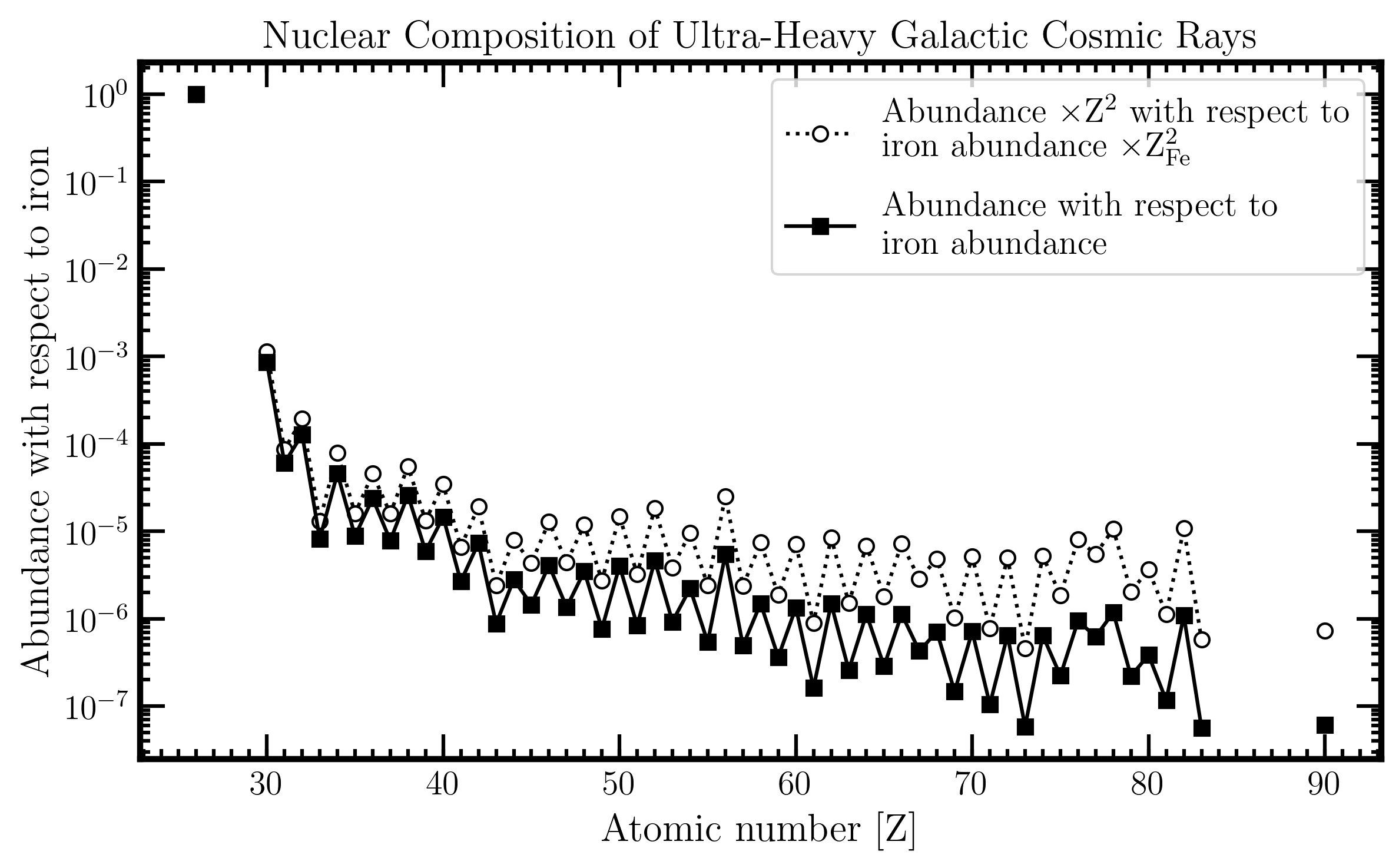
Fig. 2. Relative abundances (black-filled squares) and relative abundances multiplied by Z2 (open circles) of GCRs at 16.2 GeV/nucleon, normalized to the iron abundance, as a function of the atomic number Z. The plot ranges from copper (Z=29) to uranium (Z=92). [Figure from Boschini et al. (2024)]
Figure 2 displays the ratio of GCR abundances from copper (Z=29) to uranium (Z=92) and the iron flux at 16.2 GeV/nucleon, obtained from SPENVIS, as a function of the atomic number Z. Additionally, the relative abundances are also shown multiplied by Z2, considering that the collision energy-loss in matter at sufficiently high energies is proportional to Z2. It is observed from the plot that the total amount of energy loss experienced by UHGCRs in the matter is less than 0.5% of the iron energy loss. Therefore, the contribution of UHGCRs to the radiation hazard in space, such as the SEE rate, can be considered negligible.
Bibliography
Boschini et al (2024), Fast and accurate evaluation of deep-space galactic cosmic ray fluxes with HelMod-4/CUDA, M. J. Boschini, G. Cavallotto, S. Della Torre, M. Gervasi, G. La Vacca, P. G. Rancoita, M. Tacconi, Advances in Space Research, April 2024, In Press
Binns, W. R., Fickle, R. K., Waddington, C. J. et al. (1981) Cosmic-ray abundances of elements with atomic number 26 less than or equal to 40 measured on HEAO 3. ApJ, 247, L115–L118. doi:10.1086/183602.
Binns, W. R., Israel, M. H., Klarmann, J. et al. (1982). The abundance of the actinides in the cosmic radiation as measured on HEAO 3. ApJ, 261, L117–L120. doi:10.1086/183899
Binns, W. R., Israel, M. H., Klarmann, J. et al. (1983). Cosmic-ray abundances of Sn, Te, Xe, and BA nuclei measured on HEAO 3. ApJ, 267, L93–L96. doi:10.1086/184010.
Binns, W. R., Israel, M. H., Brewster, N. R. et al. (1985). Lead, platinum, and other heavy elements in the primary cosmic radiation - HEAO 3 results. ApJ, 297, 111–118. doi:10.1086/163508.
Binns, W. R., Garrard, T. L., Gibner, P. S. et al. (1989). Abundances of Ultra-heavy Elements in the Cosmic Radiation: Results from HEAO 3. ApJ, 346, 997. doi:10.1086/168082.
Domingo, C., Font, J., Baixeras, C. et al. (1996). Source abundances of ultraheavy elements derived from UHCRE measurements. Radiation Measurements, 26(6), 825–832. doi:10.1016/S1350-4487(96)00090-X.
Donnelly, J., Thompson, A., O’Sullivan, D. et al. (2012). Actinide and Ultra-Heavy Abundances in the Local Galactic Cosmic Rays: An Analysis of the Results from the LDEF Ultra-Heavy Cosmic-Ray Experiment. ApJ, 747(1),40. doi:10.1088/0004-637X/747/1/40.
Dutta, A., Batra, V., & Biswas, S. (2003). Abundance of actinides in cosmic radiation. Radiation Measurements, 36(1-6), 287–290. doi:10.1016/S1350-4487(03)00137-9.
ECSS (2020). Space Environment. Technical Report ECSS-E-ST-10-04C Rev.1 European Cooperation for Space Standardization, ESA. URL: https://ecss.nl/standard/ecss-e-st-10-04c-rev-1-space-environment-15-june-2020/
Fowler, P. H., Walker, R. N. F., Masheder, M. R. W. et al. (1987). Ariel Measurements of the Fluxes of Ultra-heavy Cosmic Rays. ApJ, 314, 739. doi:10.1086/165101
ISO (2004). Space Environment (Natural and Artificial) - Galactic Cosmic Ray Model. Standard International Organization for Standardization Geneva, CH. URL: https://www.iso.org/standard/37095.html.
Lingenfelter, R. E. (2019). The Origin of Cosmic Rays: How Their Composition Defines Their Sources and Sites and the Processes of Their Mixing,Injection, and Acceleration. ApJS, 245(2), 30. doi:10.3847/1538-4365/ab4b58.
Maurin, D., Dembinski, H. P., Gonzalez, J. et al. (2020). Cosmic-Ray DatabaseUpdate: Ultra-High Energy, Ultra-Heavy, and Antinuclei Cosmic-Ray Data(CRDB v4.0). Universe, 6(8), 102. doi:10.3390/universe6080102.
Maurin, D., Melot, F., & Taillet, R. (2014). A database of chargedcosmic rays. A&A, 569, A32. doi:10.1051/0004-6361/201321344.
Murphy, R. P., Sasaki, M., Binns, W. R. et al. (2016). Galactic Cosmic RayOrigins and OB Associations: Evidence from SuperTIGER Observations ofElements 26Fe through 40Zr. ApJ, 831(2), 148. doi:10.3847/0004-637X/831/2/148.
Rauch, B. F., Link, J. T., Lodders, K. et al. (2009). Cosmic Ray origin in OB Associations and Preferential Acceleration of Refractory Elements: Evidence from Abundances of Elements 26Fe through 34Se. ApJ, 697(2), 2083–2088. doi:10.1088/0004-637X/697/2/2083.
Tatischeff, V., Raymond, J. C., Duprat, J. et al. (2021). The origin of Galacticcosmic rays as revealed by their composition. MNRAS, 508(1), 1321–1345.doi:10.1093/mnras/stab2533.
Weaver, B. A., & Westphal, A. J. (2002). Extended Analysis of the Trek Ultra-heavy Collector. ApJ, 569(1), 493–500. doi:10.1086/339265.
Westphal, A. J., Price, P. B., Weaver, B. A. et al. (1998). Evidence againststellar chromospheric origin of Galactic cosmic rays. Nature, 396(6706),50–52. doi:10.1038/23887
Wiedenbeck, M. E., Binns, W. R., Cummings, A. C. et al. (2007). An Overviewof the Origin of Galactic Cosmic Rays as Inferred from Observations ofHeavy Ion Composition and Spectra. Space Sci. Rev., 130(1-4), 415–429.doi:10.1007/s11214-007-9198-y
- Details
- Hits: 4780
GALPROP obtained LIS using modulated spectra from HelMod
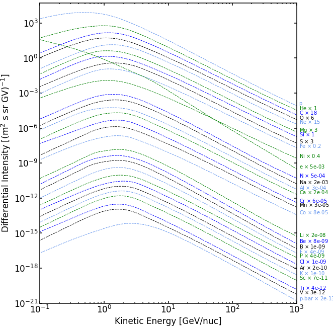
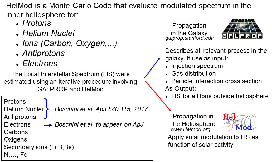
The local interstellar spectra (LIS) are input cosmic ray intensities for any modulation models. Fluxes are assumed isotropically distributed at heliosphere boundary, in a steady-state configuration. The LIS is usually computed using numerical model accounting for the propagation in galaxy. The heliosphere modulation is the added using, e.g.,the modulation module available here for on line use or download.
Recently, Boschini et al 2017, 2018a, 2018b, 2020a, 2020b deduced LIS's for protons, helium nuclei and antiprotons using the most recent experimental results combined with GALPROP model for propagation in galaxy and HelMod for the propagation in heliosphere.
Successive work extend the available sets of LIS's. Boschini et al 2018b, using the same procedure, deduced LIS's for Carbon- and Oxygen-nuclei, while Boschini et al 2018a deduced LIS for galactic electrons.
HelMod and GALPROP were combined to provide a single framework and run to reproduce a comprehensive set of observations of CR species collected in different time periods, from 1997 up to 2015.
The numerical table of computed LIS is available as supplementary material of Boschini et al 2017, Boschini et al. 2018a, and Boschini et al 2020b.
Antiproton LIS
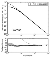
Boschini et al 2017 provides analytical fits to the derived LIS. The fit to the antiproton LIS provides an accuracy of 2-3% for 3 GV \(<R<1000\) GV and 10% for 1.5 GV \(<R<3\) GV:
\begin{equation}
F(R)\times R^{2.7} = 1.34-4.99\times 10^{-4}R+\frac{44.3}{12.6+R}-\frac{168}{31.1+R^{2}} +\frac{13600}{22200+R^{2}}, \quad R>1.5\ {\rm GV},
\end{equation}
while the average accuracy of AMS-02 data is about 10%-20%.
Electron LIS
In Boschini et al 2018a., it was provided a parameterization \(F(T)\) of the electron GALPROP LIS from 2 MeV up to 90 GeV as a function of kinetic energy in GeV:
\begin{align}\label{EQ::ele}
&F(T) = \\
&\left\{
\begin{array}{ll}
\frac{1.181\!\!\times\!\! 10^{11} T^{-12.061}}{1+4.307\!\!\times\!\! 10^{8} T^{-9.269}+3.125\!\!\times\!\! 10^{8} T^{-10.697}} & T<6.88 GeV\,\\ \nonumber
995.598\, T^{-3.505}+4.423\, T^{-2.620}, & T\ge 6.88 GeV, \nonumber
\end{array}
\right.\nonumber
\end{align}
where the units are (m\(^2\) s sr GeV)\(^{-1}\). This fit reproduces the \galprop{} electron LIS with an accuracy better than 5\% for the whole quoted energy range.
The electron LIS that results from the model calculations is in a good agreement with data (See discussion in Boschini et al 2018a.). Meanwhile, it may harbor an additional electron component from an unknown source of the same nature as that of the excess positrons. If charge-sign symmetry is assumed, i.e. that the electron and positron components coming from an unknown source have identical spectra, then the spectral shape of such an additional electron component can be derived from AMS-02 positron measurements. The spectrum of an additional component, ``the signal,'' \(S(T)\) can be parametrized as a function of kinetic energy as:
\begin{equation}
S(T)= 4.5\times10^{-3}\ T^{-1.53} e^{-\frac{T}{400\ {\rm GeV}}}\ ({\rm m}^2\ {\rm s\ sr\ GeV})^{-1}
\end{equation}
This involves a re-tuning of the electron injection spectrum above the break at 95 GV (See discussion in Boschini et al 2018a.). This parameterization also takes into account the standard astrophysical background of secondary positrons evaluated to be \(\le\)6\% at 30 GeV.
LIS for Proton and Nuclei up to Z<=28
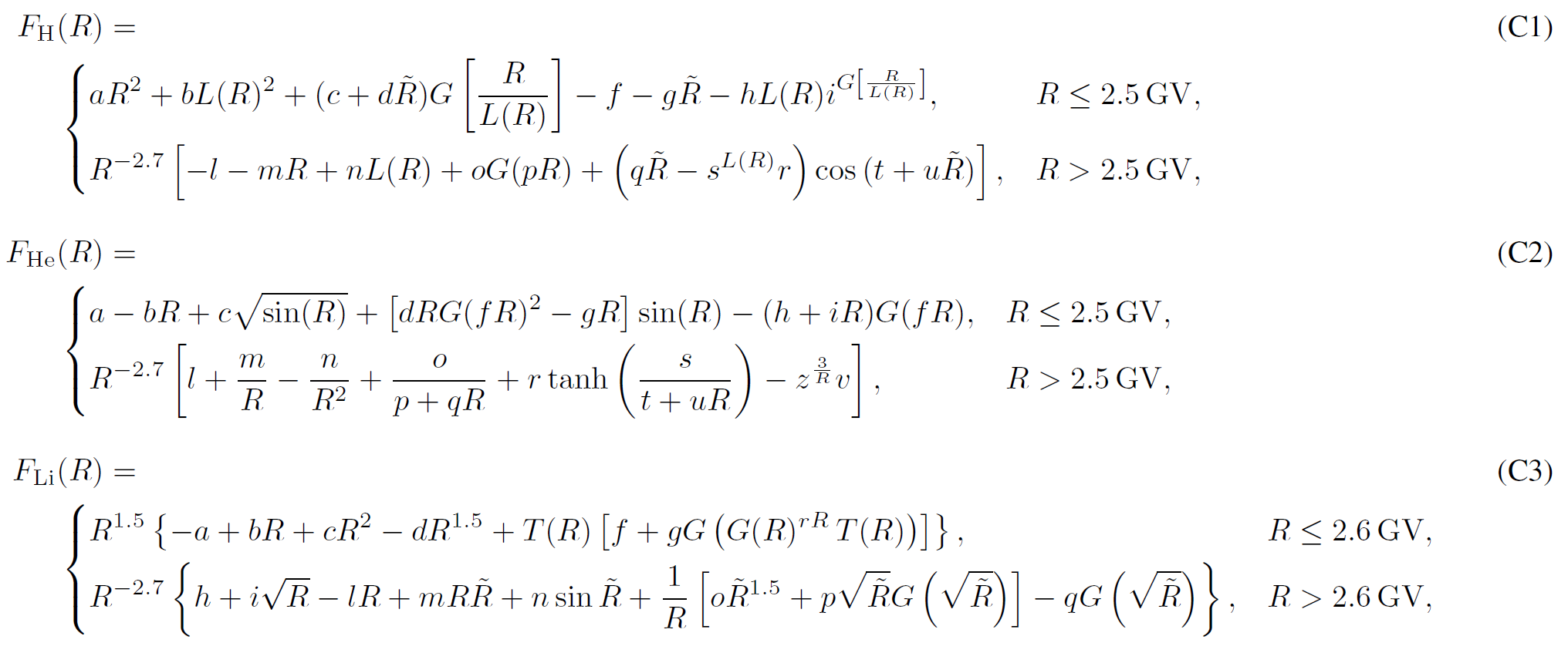
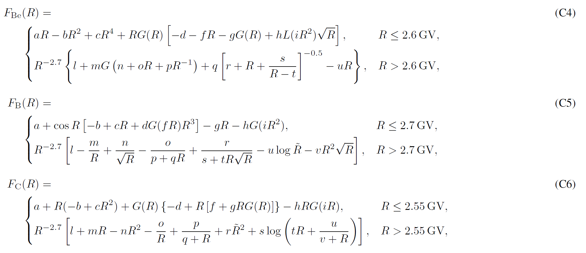
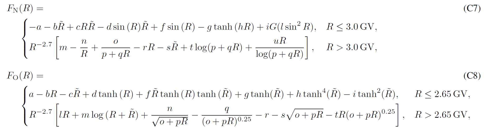
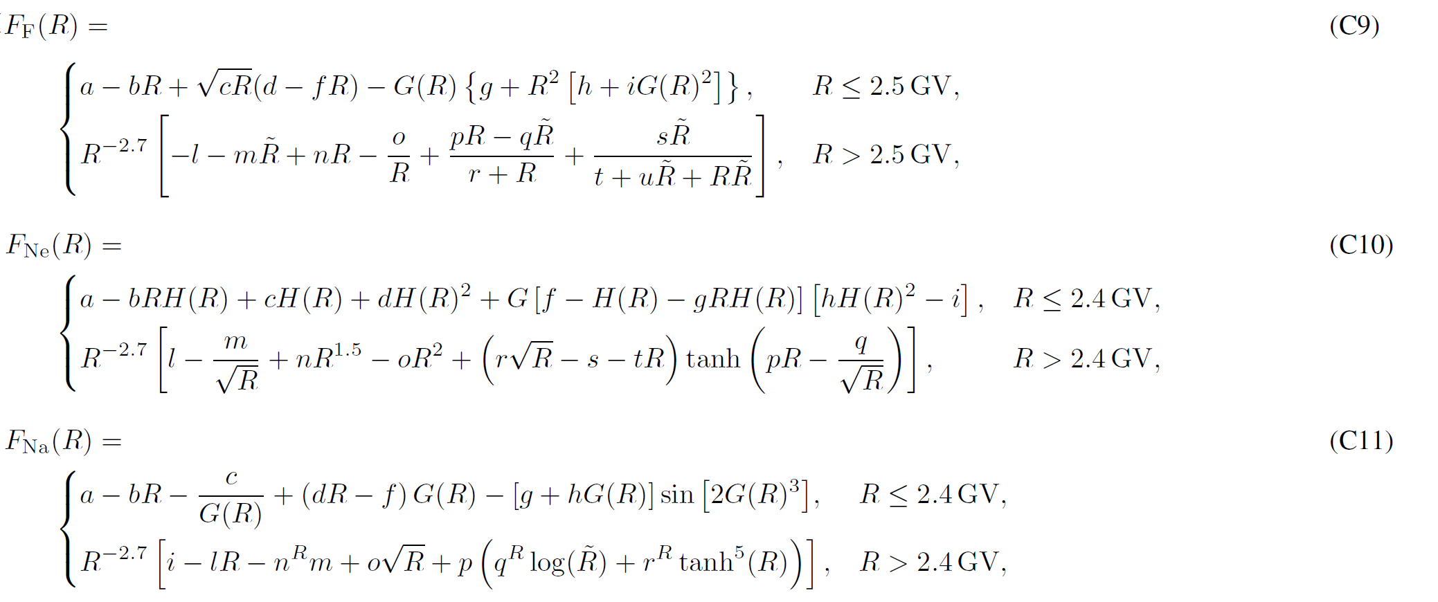
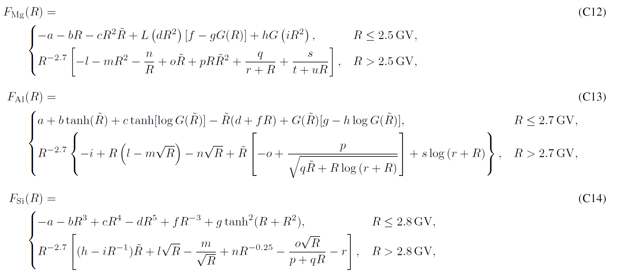
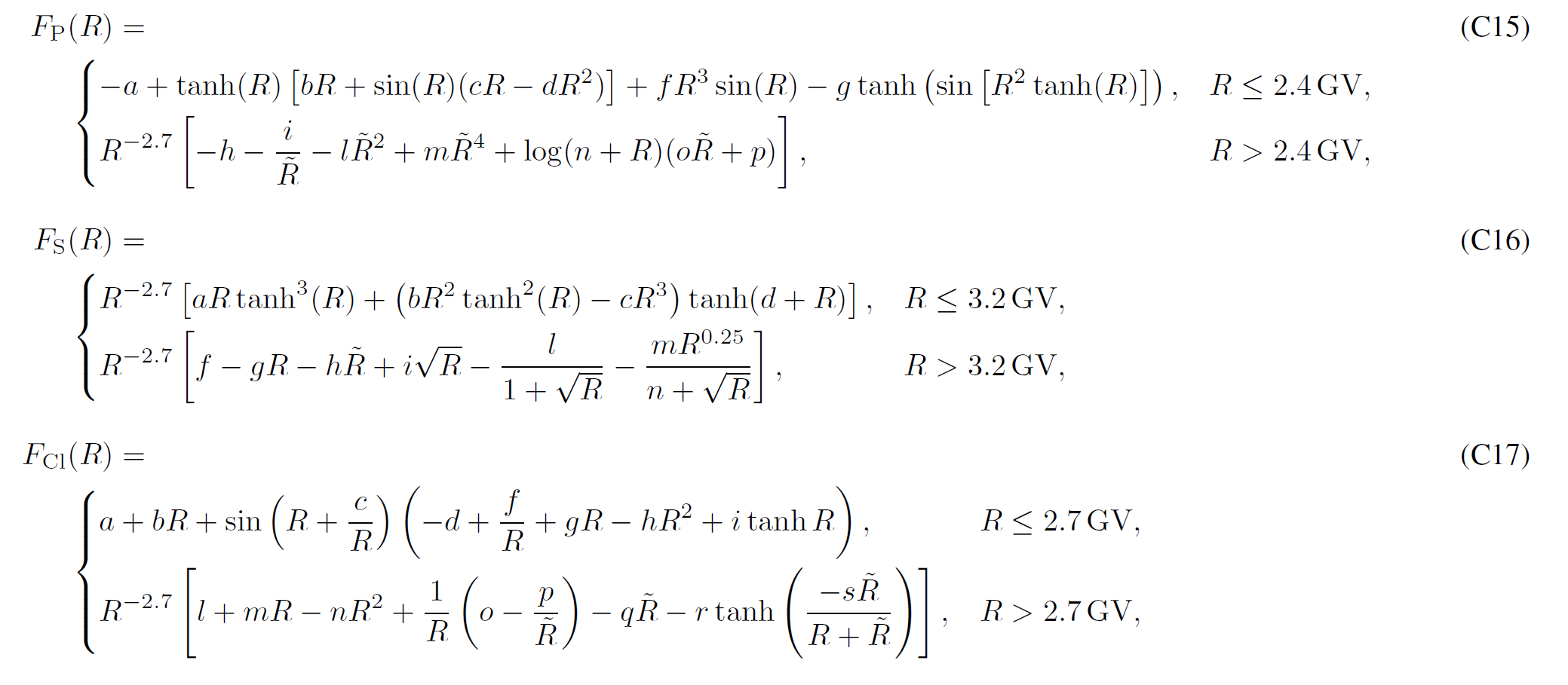
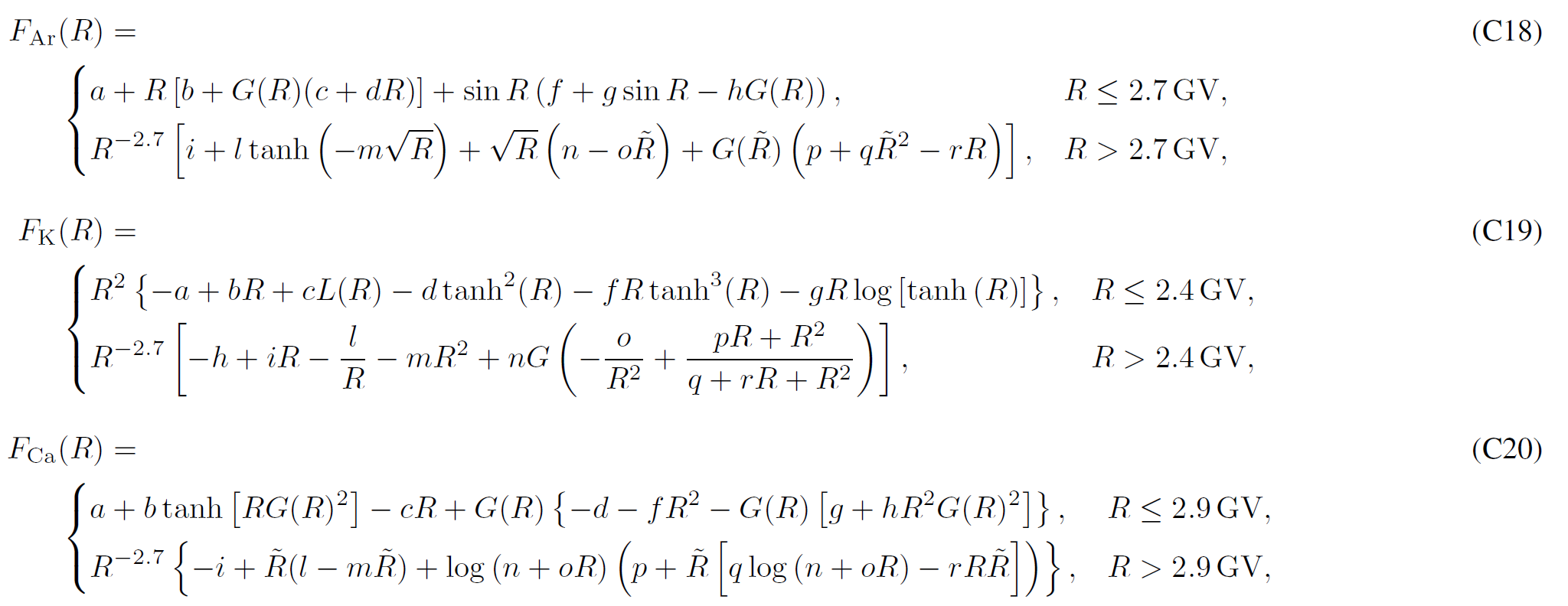
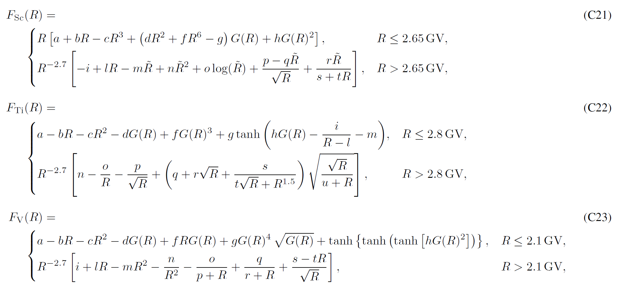
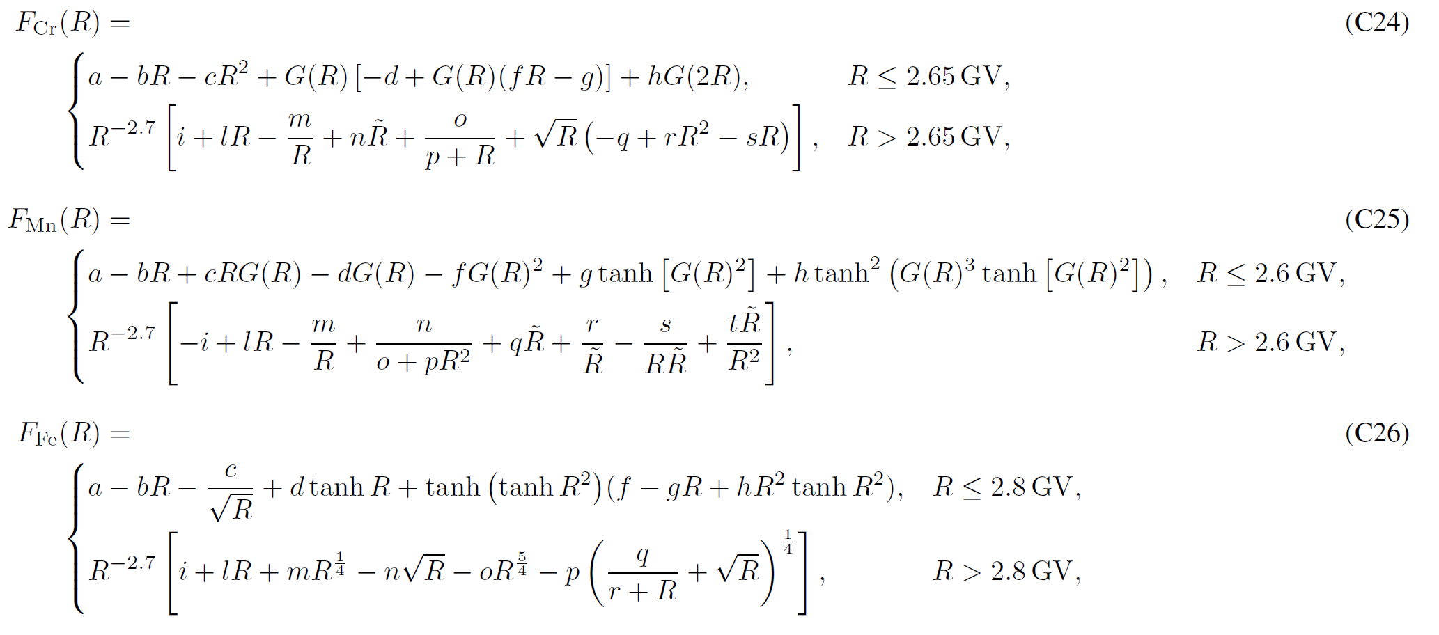
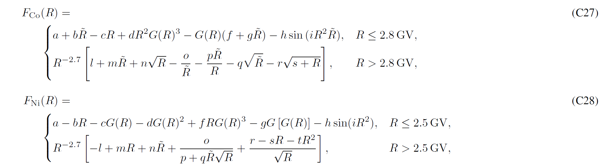
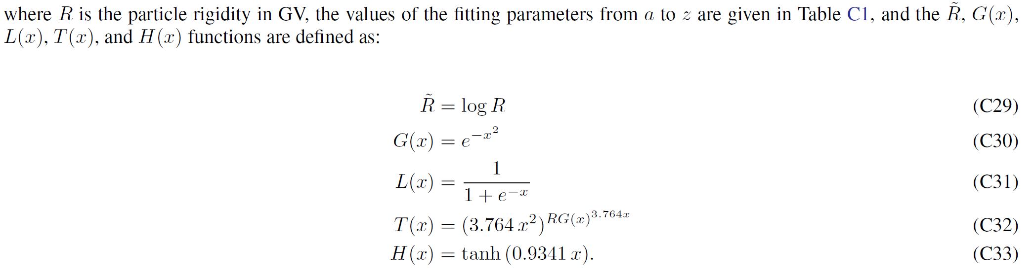
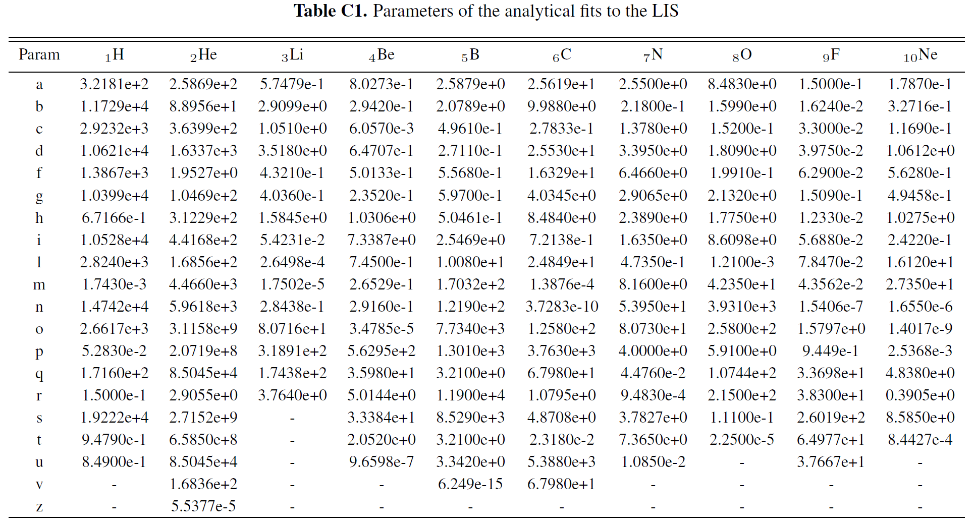
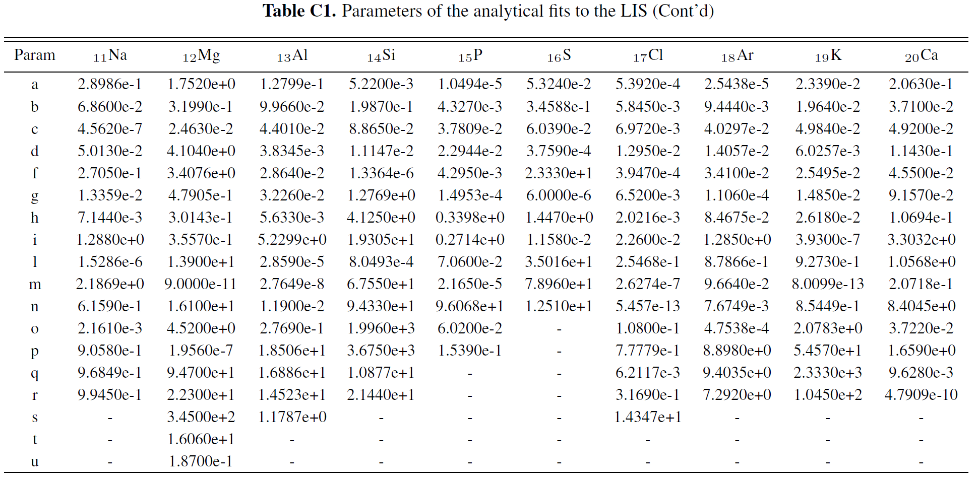
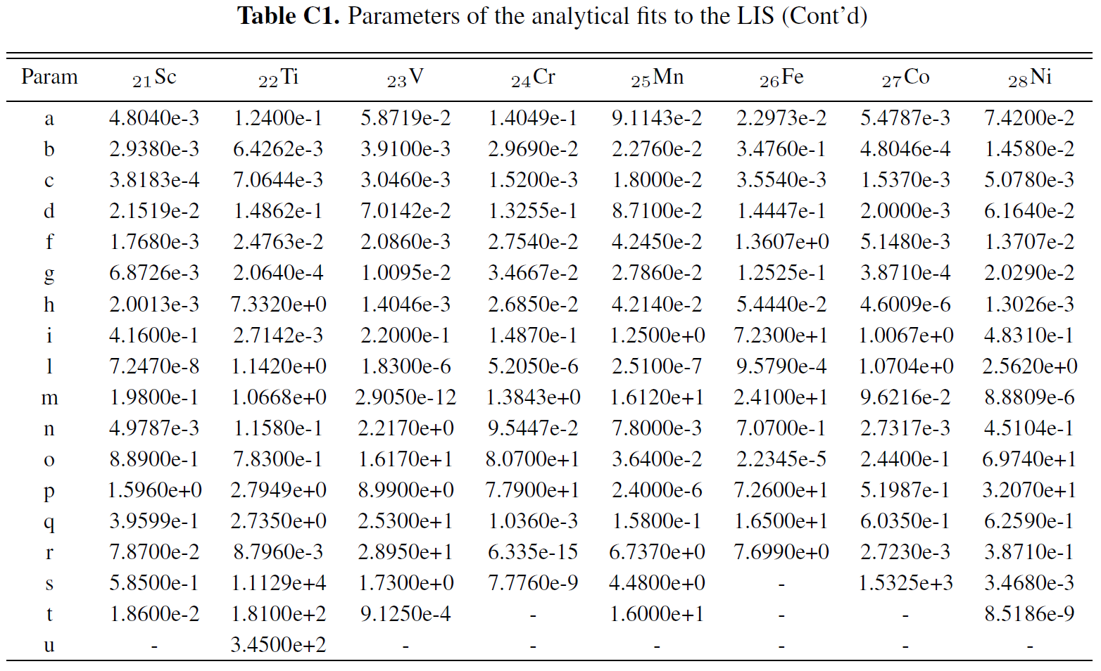
Boschini et al 2020b provide analytical parameterizations of the LIS for each species, with parameters summarized inTable C1. The presented formulas parametrize numerical LISs obtained from the join effor of GALPROP and HelMod with an accuracy below 3% from 0.1 GV up to 105 GV and complete the numerical tables.
Bibliography
- Details
- Hits: 9800
By exploiting experimental results, the combined effort of the physicists involved with the Galprop model for propagation in galaxy and HelMod for the propagation in heliosphere, the local interstellar spectra (LIS) for Galactic Cosmic Rays species up to Z=28 (Nickel) were derived. These spectra are available and accessible from the current webpage.
Some of the currently available LIS's were derived accounting for AMS-02 data published up to TV rigidity region. The exploitation of AMS-02 data allowed one to approach the procedure with high statistic data of unprecedent accuracy. Currently, the observation data at Earth on cosmic rays species from HEAO3-C2 (from october 1979 to June 1980) and AMS-02 were employed for absolute scale normalization of fluxes (see Sects. 3-3.2 in Boschini et al. 2020).
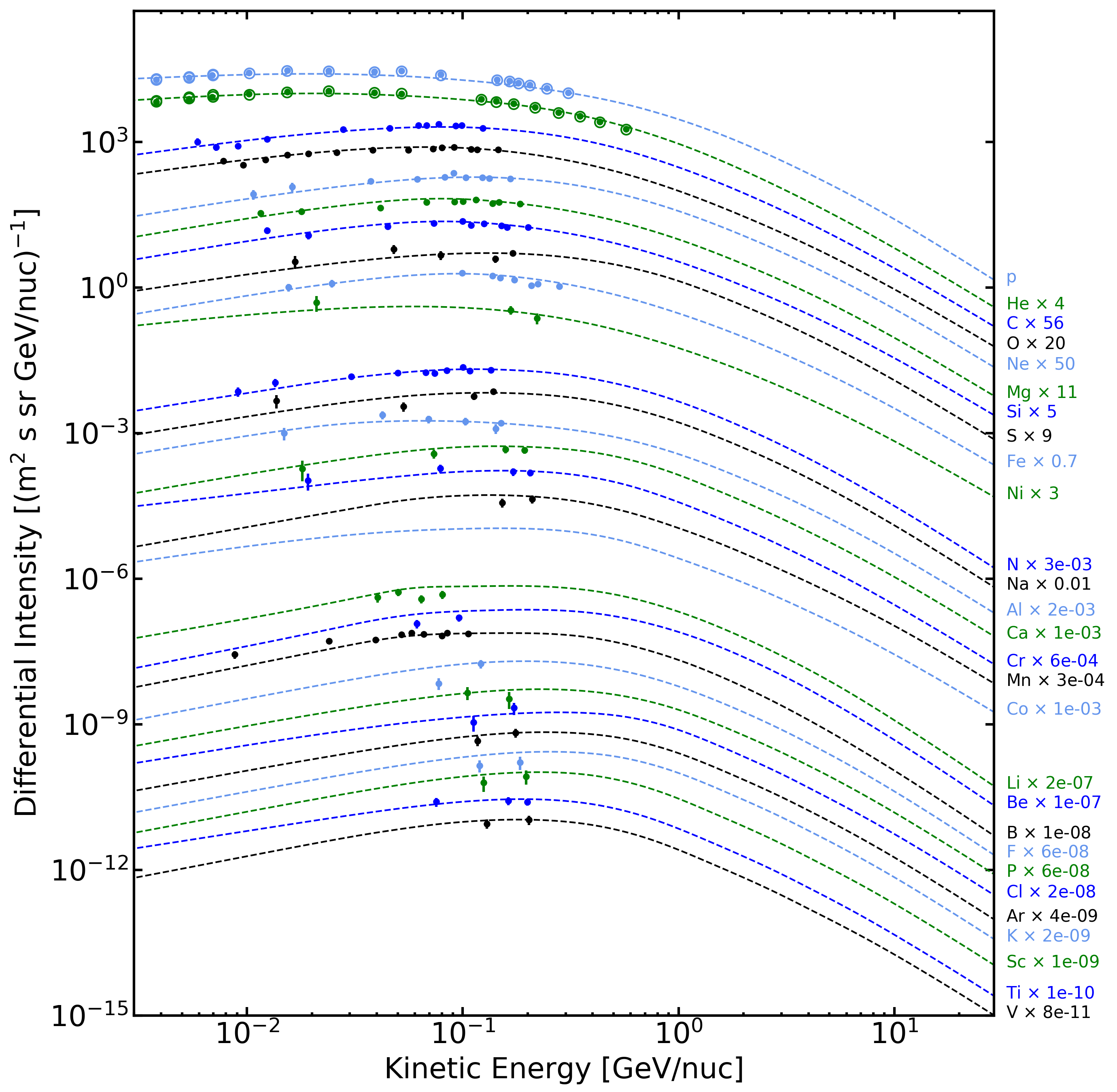 The GALPROP LIS for all CR species (dashed lines) are compared to the Voyager 1 data (filled circles, Cummings et al 2016). We also show updated Voyager 1 data for H and He (open circles) taken from September 1, 2012 to November 13, 2019. The elements are sorted by approximate amount of primary contribution: first group is mostly primary, second – with significant primary contribution, and third – mostly secondary.
 Galprop-HelMod join effort
- Details
- Hits: 11172
The following text is based on / Extracted from Boschini et al 2019 and regards HelMod version 4 and beyond.
The boundary of the heliosphere, called heliopause (HP), is a contact discontinuity separating the solar cavity -- in which the SW plasma is flowing -- from the interstellar space. It also represents the extreme limit beyond which solar modulation does not affect CR flux. Thus, outside HP the truly pristine LIS of GCR spectra could be observed. After being accelerated in the solar corona (Parker, 1958) SW adiabatically expands in radial direction with supersonic speed. In its journey towards the external regions of the heliosphere SW flow changes its supersonic regime, through the formation of a physical boundary called Termination Shock (TS) which, in practice, separates the inner part of the heliosphere1 from the outer region2, also known as heliosheath (HS).
The heliosphere boundaries (i.e., TS and HP) were extensively discussed in the literature (e.g., Parker, 1961,1963; Axford, 1972; Holzer, 1989; Zank, 1999,2015 and references therein). Recently, fundamental advancements in the knowledge of the outer heliosphere were achieved by means of both Voyager probes, which provided on-site observations of TS and HP positions, SW plasma and magnetic field properties (e.g., see Richardson et al, 2008; Richardson, 2013,Nasa-Voyager,Burlaga and Ness, 2016,Nasa-OMNIWeb). In Parker's model of the heliosphere (Parker, 1961, 1963), such pieces of information can be exploited for allowing us to estimate the time dependence of both TS and HP positions -- i.e., those currently used in HelMod --, as discussed in Heliospheric boundaries section. For instance, the predicted TS values are in good agreement with those observed: for Voyager 1 (Voyager 2) the detected TS position is 93.8 AU (83.6 AU) and the predicted is 91.8 AU (86.3 AU), i.e. within 3 AU; and, using the HP position observed by Voyager 1, the predicted value is 120.7 AU at the time of the Voyager 2 HP crossing which occurred at 119 AU. Furthermore, the interstellar magnetic field strength measured by Voyager 1 is \((0.48\pm0.04)\)nT (Burlaga e Ness, 2016). In the context of the Parker model, at the TS positions observed by Voyager 1 and Voyager 2, such a magnitude requires that the value of the dimensionless stagnation pressure (Parker, 1963) approaches its maximum value, i.e., the one allowed for a spherical diamagnetic solar cavity (see discussion in Heliospheric boundaries section). It should be remarked that, from the measurements of energetic neutral atoms by IBEX (McComas et al, 2009) and Cassini (Krimigis, 2009), Dialynas et al. (2017) strongly suggested a diamagnetic bubble-like heliosphere3 with negligibly small tail-like features (see also Drake, 2015,Opher et al 2015, 2017).
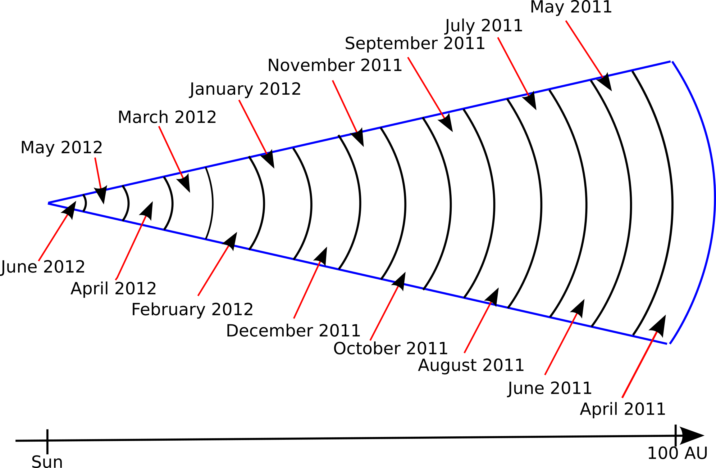
In HelMod model, so far the inner region of the heliosphere was described as an effective heliosphere (Bobik et al 2012) with a radius -- i.e., an effective TS distance -- of 100AU. Solar modulation was, then, treated by subdividing it in 15 radially equally-spaced regions. Each i-th region traveled by CR particles is characterized by heliospheric parameters evaluated at i-Carrington rotations back-in-time, corresponding to the time needed by SW for reaching it (Bobik et al 2012, Boschini et al 2018).
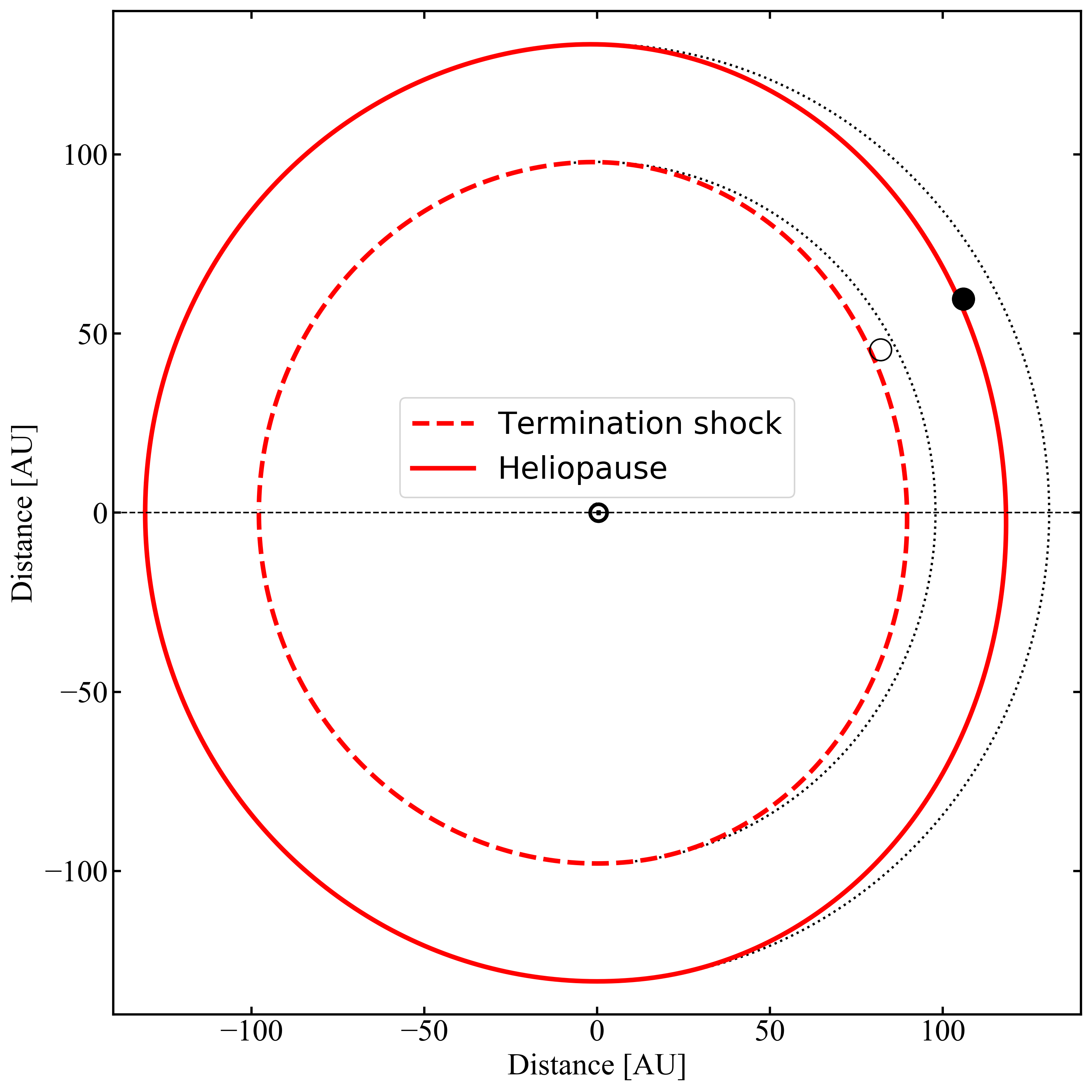
The actual dimensions of the heliosphere are accounted for by scaling the position of TS by the time dependent values obtained as described in Heliospheric boundaries section. The HS is included as a single additional region on top of the 15 inner regions with its actual size as calculated in Heliospheric boundaries section. As discussed in Heliospheric boundaries section the TS and HP latitudinal profile in the nose region was determined taking into account the latitudinal variation of the ISM ram pressure component of the total pressure on the HP surface. In the anti-nose region only the magnetic and plasma pressure were accounted for. As a consequence, an asymmetry in the direction of the ISM flow is introduced (see fig. below). Finally a cylindrical symmetry with respect to the axis along the sun-nose direction was applied to have full three-dimensional heliospheric boundaries.
1The inner part of the heliosphere -- corresponding to the space region from the Sun up to the TS -- will be indicated as inner heliosphere in the following.
2The outer part of the heliosphere - corresponding to the space region from the TS up to the HP - will be indicated as outer heliosphere in the following.
3Under the condition that there is no interstellar magnetic field, Parker, (1961; 1963) discussed the case of a steady subsonic interstellar wind leading to a comet-like shape (see, e.g., Axford, 1972; Holzer, 1989, Zank 1999, 2015 and references therein).
Bibliography
 |
Bobik, P., Boella, G., Boschini, M.~J., Consolandi, C., Della Torre, S., Gervasi, M., Grandi, D., Kudela, K., Pensotti, S., Rancoita P.G. and Tacconi, M. (2012). Systematic Investigation of Solar Modulation of Galactic Protons for Solar Cycle 23 Using a Monte Carlo Approach with Particle Drift Effects and Latitudinal Dependence. Astrophys. J., 745:132 . |
 |
Boschini, M.J., Della Torre, S., Gervasi, M., La Vacca, G. and Rancoita, P. G. (2018a) Propagation of Cosmic Rays in Heliosphere: the HelMod Model Adv. Space Res. 62(10):2859 - 2879, 2018 |
 |
Boschini, M.J., Della Torre, S., Gervasi, M., La Vacca, G. and Rancoita, P. G. (2019) The HelMod Model in the Works for Inner and Outer Heliosphere: from AMS to Voyager Probes Observations Advances in Space Research 64(12):2459 - 2476, 2019. |
| Axford, W.I., 1972. NASA Special Publication 308, 609. | |
| Burlaga, L.F., 1984. Space Sci. Rev. 39, 255–316. | |
| Burlaga, L.F., Ness, N.F., 2016. Astrophys. J. 829, 134. | |
| Dialynas, K., et al., 2017. Nature Astronomy 1, 0115. | |
| Drake, J.F., Swisdak, M., Opher, M., 2015. Astrophys. J. Letter 808, L44. | |
| Holzer, T.E., 1989. Annu. Rev. Astron. Astrophys. 27, 199 – 234. | |
| Krimigis, S.M., 2009. Science 326, 971. | |
| McComas, D.J., et al. 2009. Science 326, 959 | |
| NASA-OMNIweb, 2018. online database http://omniweb.gsfc.nasa.gov/form/dx1.html . | |
| NASA-Voyager, 2018. online database https://voyager.gsfc.nasa.gov/flux.html . | |
| Opher, M., Drake, J.F., Swisdak, M., Zieger, B., Toth, G., 2017. Astrophys. J. Letter 839, L12 | |
| Opher, M., Drake, J.F., Zieger, B., Gombosi, T.I., 2015. Astrophys. J. Letter 800, L28. | |
| Parker, E.N., 1958. Astrophys. J. 128, 664. | |
| Parker, E.N., 1961. Astrophys. J. 134, 20. | |
| Parker, E.N., 1963. Interplanetary dynamical processes. | |
| Richardson, J.D., Kasper, J.C., Wang, C., Belcher, J.W., Lazarus, A.J., 2008. Nature 454, 63–66 | |
| Richardson, J.D., 2013. Journal of AdvancedResearch 4, 229–233. | |
| Zank, G., 2015. Annual Review of Astronomy and Astrophysics 53, 449–500. | |
| Zank, G.P., 1999. Space Sci. Rev. 89, 413–688. |
- Details
- Hits: 12527