
In the most general case, the transition density function \(Q(s,y;t,x)\) from a phase-space point \(y\) at time \(s\) to a new time and position \((t,x)\), associated to an advective and a diffusive process described by moderately smooth functions, satisfy a Fokker-Plank partial differential equation [see e.g. Bobik et al., 2016 and reference there-in]. In term of differential operators, formally the backward-in-time evolution is described by the adjoint operator of the time-forward. In this approach the Kolmogorov backward equation [Kloeden & Platen, 1999] gives the backward evolution of the associated transition density function with respect to the initial state \((s,y)\) [see e.g. Bobik et al., 2016 and reference there-in]:
\begin{equation}\label{eq:FPEGeneral_Bck}
\frac{\partial Q}{\partial s} = \sum_i A_{B,i}(s,y) \frac{\partial Q}{\partial y_i}+\frac{1}{2}\sum_{i,j} C_{B,ij}(s,y) \frac{\partial^2 Q}{\partial y_i\partial y_j} -L_B Q + S
\end{equation}
where \(A_{B,i}\) is the advective term for \(i-th\) coordinate (e.g. convection due to Solar Wind and Magnetic Drift), \(C_{B,ij}\) is the diffusion tensor, \(L_B\) describes (catastrophic) ``losses'' and finally \(S\) describes ``source'' of particles. We underline that \(\partial s>0\) represents a propagation backward-in-time.
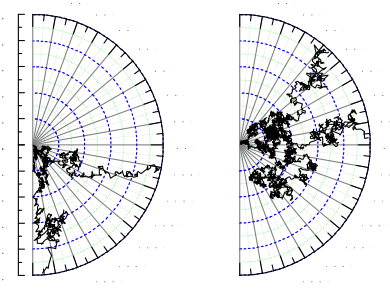
We solved Parker Equation using the backward-in-time approach using the newest version of HelMod Code. The numerical approach is to solve a set of Stochastic Differential Equation (SDE) fully equivalent to a FPE in the form of Eq.\eqref{eq:FPEGeneral_Bck}. As many authors underlines [see e.g.Bobik et al., 2012;Bobik et al., 2016 and reference there-in], this approach allows for more flexibility in model implementation, more stability of numerical results and to explore physical results that are hard to handle with ``classical'' numerical methods. With the Monte Carlo approach, the solution can be evaluated computing the SDE ``forward-in-time'' and ``backward-in-time''. In ``forward-in-time'' approach quasi-particle objects were traced in the heliosphere from the heliosphere boundary down to the inner heliosphere. In ``backward-in-time'' approach the numerical process starts from the target and trace-back quasi-particle objects till the heliosphere boundary.
The equivalence between the two methods were discussed in Bobik et al., 2016.
In terms of SDEs, the evolution of the stochastic process can be described by:
\begin{equation}\label{eq::SDEGeneral_Fwd}
dx_i(t) = A_{B,i}dt+B_{B,i,j}dW_j(t),
\end{equation}
where \(\vec C_{B}=\tilde B_{B}\tilde B_{B}^T \), \(d\vec{W}\) represents the increments of a \emph{standard Wiener process} that can be represented as an independent random variable of the form \(\omega_j \sqrt{d t} \) and, finally, \(\omega_j\) denotes a normally distributed random variable with zero mean value and unit variance.
To evaluate SDEs the Parker Equation should be rewritten in the form of Eq.\eqref{eq:FPEGeneral_Bck}. The set of the approximated SDEs, for a 2-dimensional approximation (radial distance and colatitude), can be represented in terms of the increments - \(\Delta r\), \(\Delta \theta\), \(\Delta T\) and \(\Delta t\),
\begin{eqnarray}
\label{2D_SDE} \Delta r &=& \left[\frac{1}{r^2}\frac{\partial r^2K_{rr}}{\partial r} +\frac{1}{r\sin\theta}\frac{\partial}{\partial \theta}\left(\sin\theta K_{\theta r}\right) - V_{sw} - V_{dr} \right]\Delta t \nonumber\\
& &+ \omega_r\sqrt{2K^S_{rr}\, \Delta t\,} , \\
\label{2D_SDE_2}\Delta \theta &=& \left[\frac{1}{r^2}\frac{\partial rK_{r\theta}}{\partial r} + \frac{1}{r\sin\theta}\frac{\partial}{\partial\theta}\left(\frac{K_{\theta \theta}\sin\theta}{r}\right)- \frac{V_{d\theta}}{r}\right]\Delta t\nonumber\\
& & + \omega_{r}\frac{2\,K_{\theta r}}{r\sqrt{2\,K_{rr}}}\sqrt{\Delta t\,}
+ \omega_{\theta}\sqrt{\frac{2}{r^2}\left( K_{\theta\theta} - \frac{K^2_{\theta r}}{K_{rr}} \right) \Delta t\,}, \\
\label{2D_SDE_3}\Delta T &=& \frac{2}{3} \frac{\alpha_{\rm rel} V_{\rm sw} T}{r} \Delta t,\\
\label{2D_SDE_4}L_B &=& \frac{2 V_{sw}}{r} \left[ \frac{1}{3} \frac{ T^2+2TT_0+ 2T_0^2 }{ (T+T_0)^2 } -1 \right ]
\end{eqnarray}
where \(\omega_{r}\) and \(\omega_{\theta}\) represent two independent gaussian distributed random number.
The vector \(\mathbf q=(r,\mu,T)\) represent a so-called pseudoparticle that evolves from target, i.e. Earth Orbit, backward to the heliosphere Border.
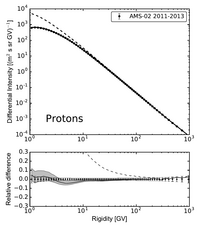
In term of stochastic simulation the modulated spectrum is obtained for each energy bin by the average of the LIS values at boundary reconstructed energy [Bobik et al., 2016]
\begin{eqnarray}
U_{detector}(T_{detector}) = \frac{1}{N}\sum_{k=1}^N U_{LIS}(r_{bound},T)\cdot \exp\left( -\sum_{j=0}^m L_{B,j} \cdot \Delta t \right)
\end{eqnarray}
where \(N\) is the number of generated quasi-particle objects with initial Energy \(T_{detector}\) (momentum \(p_{detector}\)), \(m\) is the number of step occurred during the stochastic propagation if \(k\)-th quasi-particle and \(r_{bound}\) is the exit point of stochastic path, i.e. the heliosphere boundary.
Differential Intensity \(J\) is finally obtained from \(J=\frac{v \mathrm{U}}{4\pi}\).
Bibliography
 |
Bobik, P., Boella, G., Boschini, M.~J., Consolandi, C., Della Torre, S., Gervasi, M., Grandi, D., Kudela, K., Pensotti, S., Rancoita P.G. and Tacconi, M. (2012). Astrophys. J., 745:132 . |
 |
Bobik, P., Boschini, M.~J., Della Torre, S., Gervasi, M., Grandi, D., La Vacca, G., Pensotti, S., Putis, M., Rancoita, P.G., Rozza, D., Tacconi, M., and Zannoni, M. (2016). J. Geophys. Res. (Space Physics), 121, 3920–3930. |
| Klöden, P. E., and E. Platen (1999), Numerical Solution of Stochastic Differential Equations, Springer, Berlin. |