
The following text is based on / Extracted from Boschini et al 2019 and regards HelMod version 4 and beyond.
The analytical modelization of the heliosphere dates back to Parker (1961) (see also discussions in Parker, 1963). In the framework of Parker's model the position of the termination shock (TS) is obtained from hydro-dynamicalconsiderations. The main hypothesis is that the heliopause (HP) is a contact discontinuity (e.g., see Suess, 1990) separating the region in which the propagation of the solar wind (SW) dominates from the interstellar medium1 (ISM). In such a model, the SW flows along streamlines from the inner part of the heliosphere, passing through theTS and traversing the heliosheath (HS) up to the stagnation point2 (with \(P_{\rm ISM}\) as stagnation pressure) on the HP in a one-dimensional radial approximation. Assuming a spherical heliocentric geometry, the SW is treated as an ideal gas3 with adiabatic index \(\gamma\) expanding steadily, radially and adiabatically towards the TS. Before reaching the TS, the largely dominant contribution to the total SW pressure4 is provided by the ram pressure \(p_{ram}=\rho u^2\), where \(\rho\) is the plasma density and \(u\) the SW speed. Moreover, for a constant SW speed up to the TS (Parker, 1958) and from the mass conservation, one finds that the plasma density (and the ram pressure) scales with distance as
\begin{align}
\rho(R)&=\rho_{obs}(R_{obs}/R)^2, \label{RscaleRho}
\end{align}
where the subscript \(obs\) refers to the quantities measured by an observer located at the heliocentric distance \(R_{obs}\).
As discussed in Parker (1961), before reaching the stagnation point, the SW must go through a shock transition: SW plasma abruptly slows down and is compressed, so that density increases5. For a shock occurring in a plane
perpendicular to the direction of flow6 (normal shock) -- as discussed for the SW shock by Parker (1961, 1963) --, the hydrodynamical quantities in the neighborhood of the shock are connected by the Rankine-Hugoniot relations (e.g. see chapter 9 in Landau and Lifshitz, 1959) which in the strong shock limit (i.e., for high Mach numbers) allow one to provide, for instance, the relationship between particle density, SW velocity and ram pressure at TS, immediately before and immediately after the shock occurrence:
\begin{eqnarray}
p_{ram\,2TS} &=&\rho_{2TS}u_{2TS}^2 \label{RH.pres2}\\
&=&\frac{\gamma-1}{\gamma+1} p_{ram\,1TS}; \label{RH.pres}
\end{eqnarray}
in the above expressions (and in the following) subscript \(1TS\) (\(2TS\)) refers to quantities just before the TS occurs (just after the TS has occurred).
The Parker hypothesis of strong shock proved to be a fairly good approximation also in light of the on-site plasma measurements by Voyager 2 probe. In fact, the Mach number can be estimated using temperature and SW speed; one finds that its value is about 9 (Richardson et al., 2008) just before the TS (i.e., at 83.6 AU) using the data from Voyager 2 (NASA-OMNIweb, 2018).
Furthermore, using the same source of data, the mean ram pressure calculated in the 2 AU before reaching the TS zone7 located at 83.6 AU is \(3.26\times10^{-4}\)nPa, while in the 2 AU after the TS zone is \(0.83\times10^{-4}\)nPa. Therefore their ratio is about 3.9 and it is in agreement with the value 4% \(\left(=\frac{\gamma+1}{\gamma-1}\right)\) -- expected for a strong shock of a monoatomic gas (e.g., see Eq. \eqref{RH.pres}) -- which, in the Parker model, provides the ratio of \(1/7{\sim}14.3\%\) (e.g., see Parker, 1961) between kinetic pressure8 and the stagnation pressure9.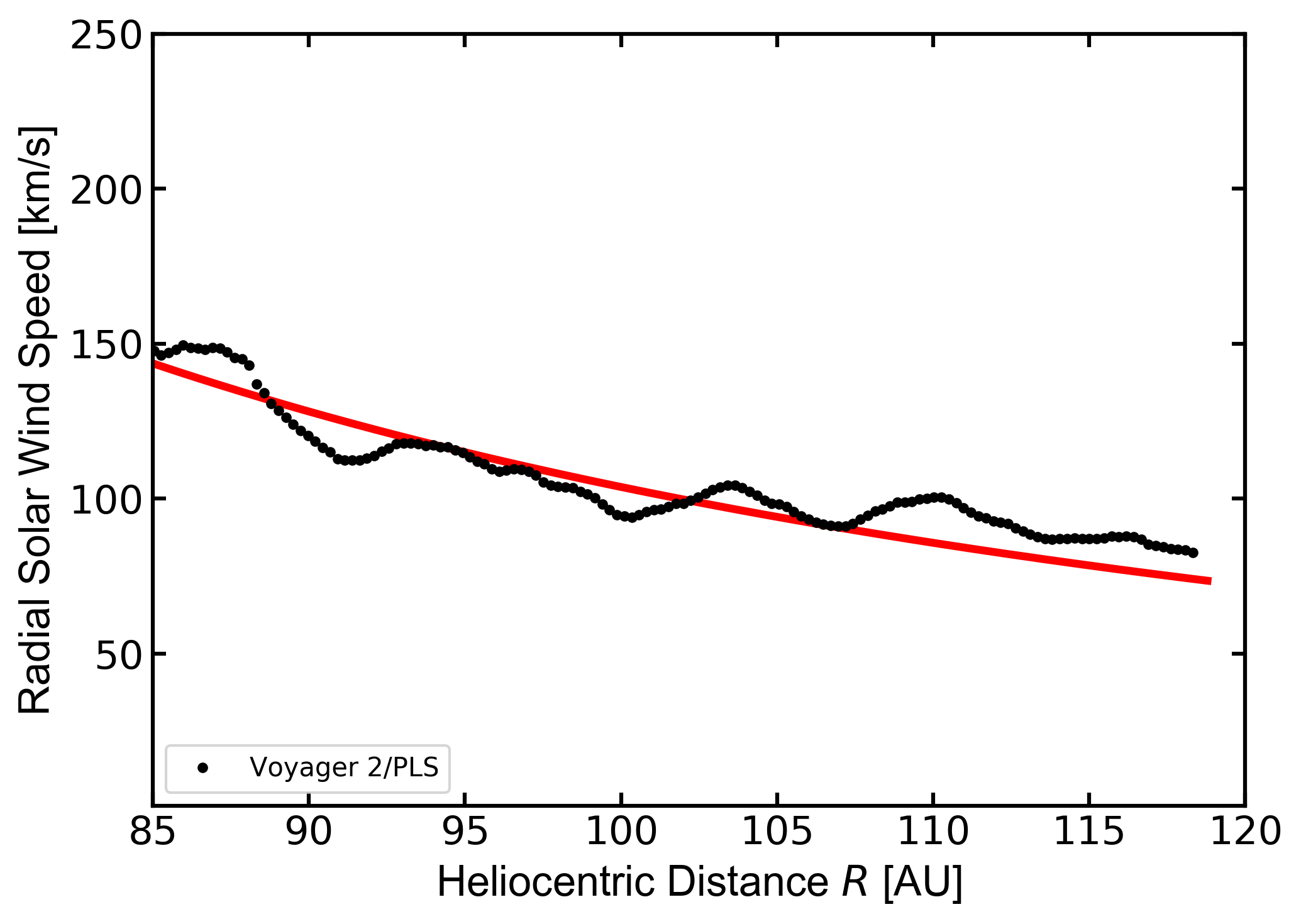
Figure 1: Radial component of the SW speed in the HS (\(V_{{\rm sw},2r}\)) as function of the heliocentric distance \(R\) downstream the Voyager 2 TS: the data are obtained with a coordinate transformation (e.g., see Burlaga, 1984) from the data in NASA-OMNIweb (2018); the solid line is the \(1/R^2\) behavior (see text). [Figure from Boschini et al 2019]
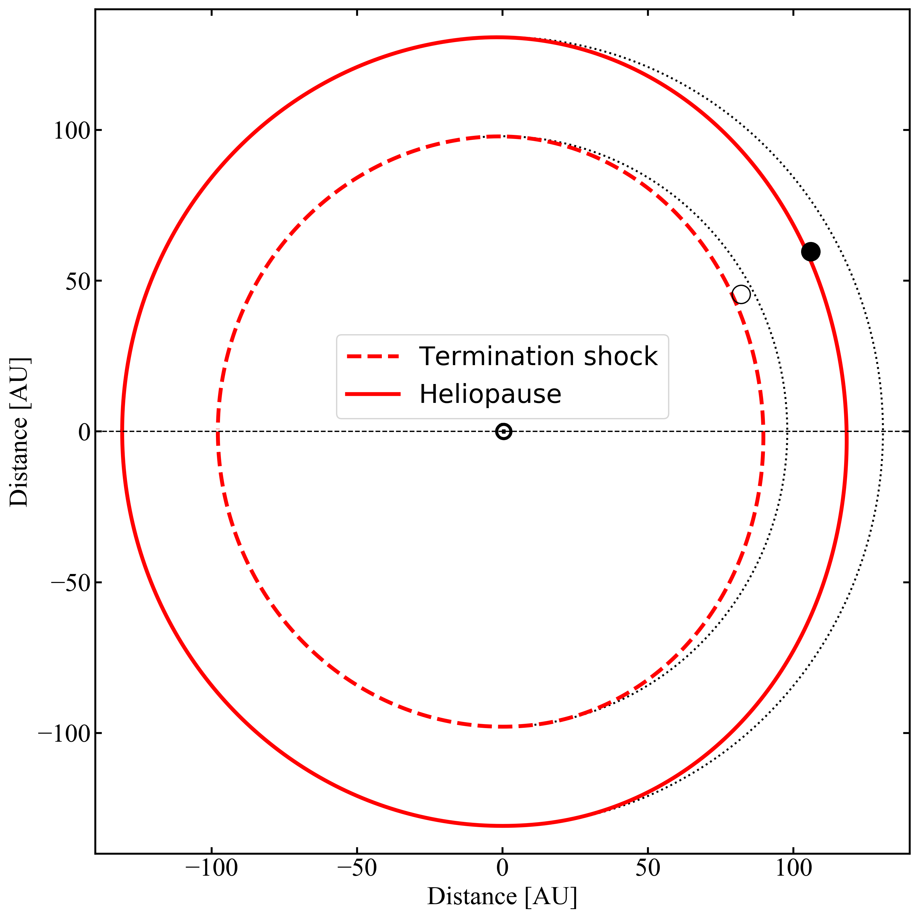
Figure 2: Meridian section of the heliosphere as described in Eq. \eqref{HelmodBoundaries}. The dashed (solid) line shows the latitudinal profile of the TS (HP) at the time and HCI latitude of the Voyager 1 TS (HP) crossing. The open (full) circle denotes the instantaneous position of Voyager 1 at TS (HP) crossing. [Figure from Boschini et al 2019]
In addition, although the SW speed in the HS does not exhibit an appreciable dependence on \(R\) (Richardson,2013), in the region downstream the TS, its radial component (\(V_{{\rm sw},2R}\)) progressively slows down flowing in the HS towards the stagnation point (Langner et al., 2003;Richardson and Decker, 2015). In Fig. 1, the radial SW speed (full circle) is obtained with a coordinate transformation (e.g., see Burlaga, 1984) from the data in NASAOMNIweb (2018). Such a decrease is compatible with the \(1/R^2\) behavior (the solid line) given by:
\begin{equation}
V_{{\rm sw},2R}(R) = u_{2TS} \left( \frac{R_{TS}}{R} \right)^2,
\label{speed.incompr}
\end{equation}
where \(u_{2TS}=150.7\) km/s (the SW speed average value calculated in the 2 AU after reaching the TS zone) and \(R_{TS}=83.6\) AU, i.e. the position of the TS observed by Voyager 2.
In the Parker model, the TS position is determined as the distance (\(R_{TS}\)) at which the total pressure in the region downstream the shock is equal to the ISM stagnation pressure \(P_{\rm ISM}\). Parker, 1961 derived two expressions for the TS position depending on whether the expansion of the shocked SW in the HS occurs through an isentropic (i.e., reversible adiabatic) or an incompressible expansion. Numerically the relative difference between those two approaches is less than \(0.4\%\) for a monatomic gas; for an incompressible flow (i.e., with plasma density \(\rho =\) const) one finds that the expression for \(R_{TS}\) is given by:
\begin{equation}
R_{TS} = R_{obs} \left( \frac{\rho_{obs} u_{obs}^2}{P_{\rm ISM}}
\right)^{\frac{1}{2}} \left[ \frac{\gamma+3}{2(\gamma+1)}
\right]^{\frac{1}{2}}.
\label{RTS.incompr}
\end{equation}
It has to be remarked that the \(P_{\rm ISM}\) determines the physical conditions for which the shock occurs at \(R_{TS}\), i.e., the inner boundary of the HS. In general, in the HS, the hydrodynamical quantities and its boundaries (TS and HP) are related to \(P_{\rm ISM}\). Voyager 1 has provided the first on-site observation of HP position (121.6 AU on Aug 2012) which allows one to determine, for instance, the value of the outward radial ram pressure of the SW at the outer heliospheric boundary.
In the Eq. \eqref{RTS.incompr}, the SW ram pressure depends on the solar activity, while \(P_{\rm ISM}\) (discussed later) is commonly assumed to be time independent. Therefore, \(R_{TS}\) can be determined as function of time using the monthly averages of the SW plasma parameters measured by various satellites (e.g., Voyager 2, Wind, ACE, Ulysses) along the last 60 years (NASA-OMNIweb, 2018; UFA, 2018). The mean value of those monthly averages finally provides the monthly estimate of \(R_{TS}\)10 (currently used in HelMod). In Eq. \eqref{RTS.incompr} the values of \(\rho_{obs}\) and \(u_{obs}\) are found taking into account the time lag (\(\Delta t_{TS}\)) needed to the SW to travel from the observation point at \(R_{obs}\) to \(R_{TS}\), i.e.,
\begin{align}
\Delta t_{TS}&=\int_{R_{obs}}^{R_{TS}} \frac{dR}{V_{\rm sw}(R)}, \label{eq:TimeDelay}\\
&=\frac{R_{TS}-R_{obs}}{u_{obs}},\label{eq:TimeDelayTS}
\end{align}
where Eq. \eqref{eq:TimeDelayTS} is employed for a constant SW speed11 equal to \(u_{obs}\). It must be remarked that using the out-of-ecliptic data from Ulysses the computed SW ram pressure apparently does not show a latitudinal dependence. In fact, at high latitudes the SW density decrease is almost completely compensated by the SW speed increase. The so calculated ram pressures are well compatible with those obtained with the data from the other satellites within the monthly fluctuations. Therefore, \(R_{TS}\) does not exhibit observable latitudinal dependencies.
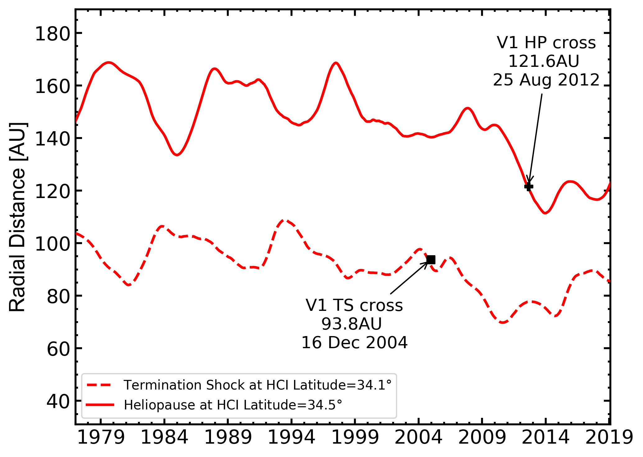
Figure 3: Time variation of monthly averaged position of TS (dashed line) and HP (solid line), calculated from 1977 up to the end of 2018. TS is calculated at HCI-latitude \(34.1°\), while HP at HCI-latitude \(34.5°\) to match Voyager 1 trajectory. The predicted TS distance at the time of Voyager 1 crossing is 91.8AU. [Figure from Boschini et al 2019]
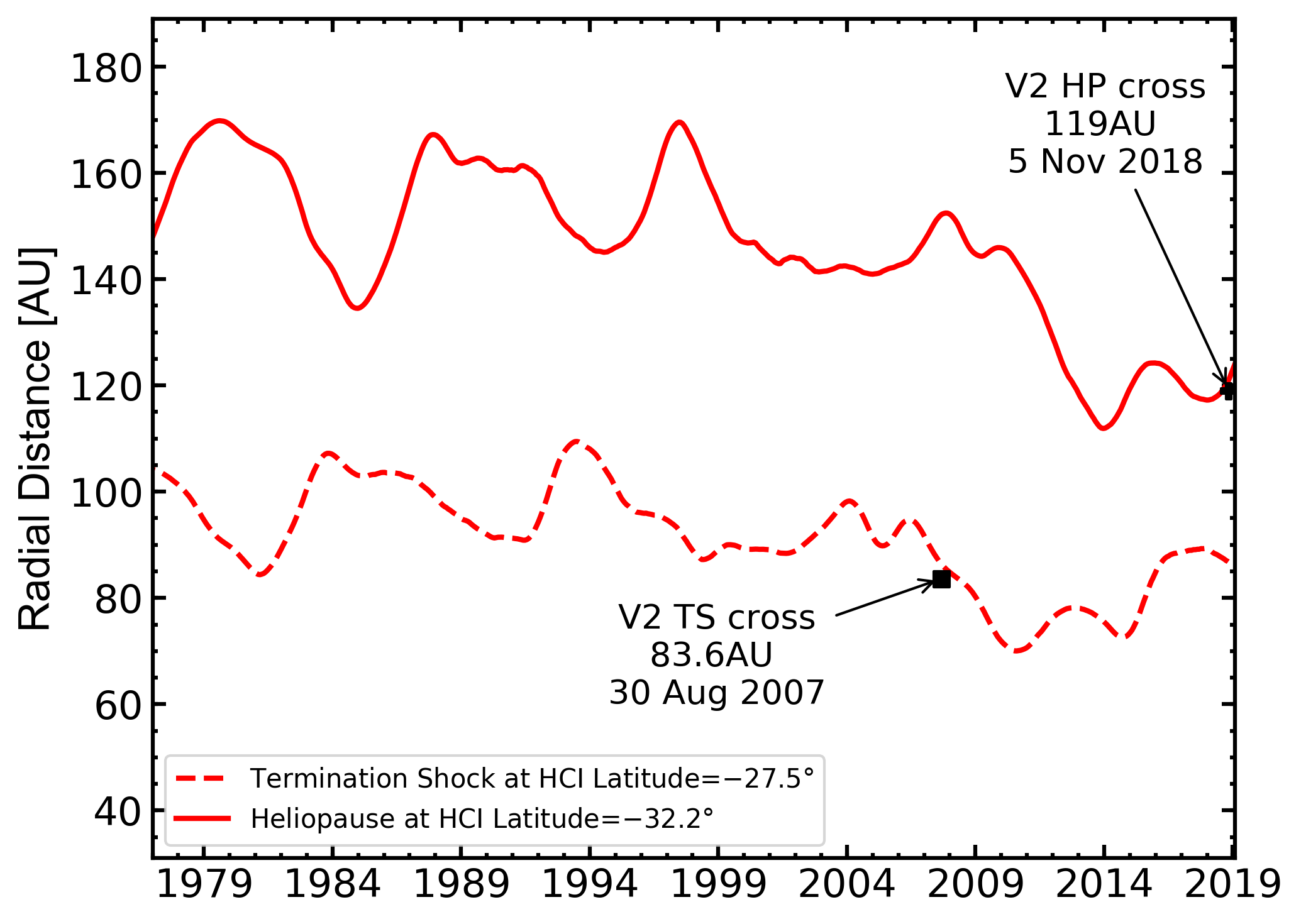
Figure 4: Time variation of monthly averaged position of TS (dashed line) and HP (solid line), calculated from 1977 up to the end of 2018. TS is calculated at heliolatitude \(-27.5°\), while HP at heliolatitude \(-32.2°\) to match trajectory of Voyager 2. The predicted TS distance at the time of Voyager 2 crossing is 86.3AU, while the predicted HP distance at the time of Voyager 2 crossing is 120.7AU. [Figure from Boschini et al 2019]
The other quantity appearing in Eq. \eqref{RTS.incompr} is the stagnation pressure \(P_{\rm ISM}\). As already discussed by Parker (1963)
(see also Parker, 1961), to a first approximation \(P_{\rm ISM}\) can be estimated by adding the interstellar (IS) magnetic field pressure (\(p_{\rm mag}\)), the kinetic pressure due to IS wind (\(p_{\rm kin}\)), the thermal pressure of the IS plasma (\(p_{\rm th}\)), i.e.,
\begin{equation}
P_{\rm ISM}=p_{\rm mag}+p_{\rm kin}+p_{\rm th}.
\label{TotISM}
\end{equation}
The values for \(p_{\rm kin}\), \(p_{\rm th}\) and \(p_{\rm mag}\) are discussed in the following (e.g. see Eqs. (\ref{pkin}, \ref{pth}, \ref{pmag_val})).
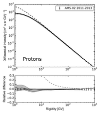
A lower contribution to \(P_{\rm ISM}\) is expected from the CR pressure (\(p_{\rm CR}\)). As already discussed by Parker (1963), \(p_{\rm CR}\) accounts for the difference between the pressure derived from the CR omnidirectional intensity in the IS space outside the HP with respect to that one obtained by the CR omnidirectional intensity immediately inside the HP. The CR pressure is determined as in Ip and Axford (1985) (see also references therein) integrating the CR particle density \(U(T)\) for protons and helium nuclei (these two species constitute the dominant contribution to the overall CR omnidirectional intensity). Their intensities immediately inside the HP are obtained from the modulated HelMod spectrum in the HS region close to the HP. The value found for \(p_{\rm CR}\) is about \(2.4\times10^{-6}\) nPa, i.e., it is of the order or lower than 1 % of the overall \(P_{\rm ISM}\) and can be neglected. The dominant contribution to the stagnation pressure comes from the IS magnetic field pressure (e.g., see equation (9.27) of Parker, 1963):
\begin{equation}
p_{\rm mag}=\Pi^2\frac{B_{\rm ISM}^2}{2 \mu_0},
\label{pmag}
\end{equation}
where \(B_{\rm ISM}\) is the average IS magnetic field magnitude, \(\mu_0\) is the permeability of free space, and \(\Pi^2=2.25\) is the dimensionless stagnation pressure (see Parker, 1963). In Parker's model, this value is the maximum allowed for \(\Pi^2\) parameter, and corresponds to an heliosphere described as a spherical "diamagnetic'' region of radius \(l\) in which the SW is streaming away from it along two opposite channels of radius \(c\rightarrow0\) along the IS magnetic field direction (e.g., see Figure 9.3 in Parker, 1963). In addition, the radius of the boundary between the IS magnetic field and the SW, i.e. the heliopause, overlaps that one of the "diamagnetic'' region.
The IS wind pressure (\(p_{\rm kin}\)) is due to the relative motion of the heliospheric cavity with respect to the ISM. In the HCI reference system12 this flow occurs close to the x-axis direction and determines the heliospheric nose direction13 ; \(p_{\rm kin}\) is given by
\begin{eqnarray}
p_{\rm kin}&=&\frac{1}{2} n_{\rm ISM} m_p \left[v_{\rm ISM}\cos(\alpha)\right]^2, \label{pkinalp} \\
&=&0.40\times10^{-4}\cos^2(\alpha) {\rm nPa},
\label{pkin}
\end{eqnarray}
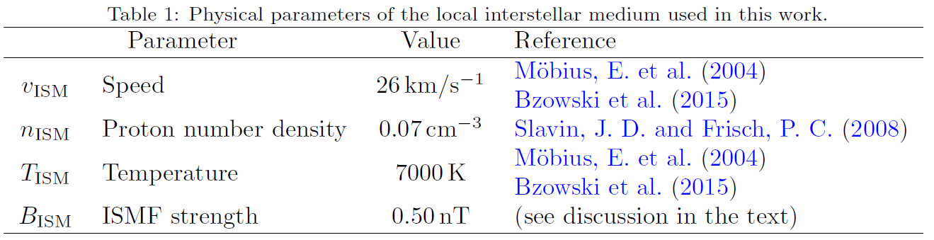
where \(n_{\rm ISM}\) (see Table 1) is the proton number density14, \(m_p\) is the proton mass, \(v_{\rm ISM}\) (see Table 1) the relative IS wind speed and, finally, \(\alpha\) is the difference between the HCI heliolatitude of the nose and the heliolatitude of the point at which the pressure is calculated. In Eq. \eqref{pkinalp}, \(v_{\rm ISM}\cos(\alpha)\) is the IS velocity component normal to the HP boundary. A further contribution comes from the thermal pressure of the interstellar plasma (\(p_{\rm th}\)):
\begin{eqnarray}
p_{\rm th}&=&2\,n_{\rm ISM} k_B T_{\rm ISM}, \nonumber\\
&=&0.14\times10^{-4} {\rm nPa},
\label{pth}
\end{eqnarray}
where \(k_B\) is the Boltzmann constant, \(T_{\rm ISM}\) (see Table 1) is the ISM temperature and \(n_{\rm ISM}\) is its number density; the factor 2 accounts for the equal amount of protons and electrons.
The first on-site observation of \(R_{TS}\) at 93.8 AU was provided by Voyager 1 on 16 December 2004. We have to remark that, since \(R_{TS}\) depends on the actual value of \(P_{\rm ISM}\) (Eq. \eqref{TotISM}) whose dominant term is \(p_{\rm mag}\) (Eq. \eqref{pmag}), at the date of Voyager 1 crossing we can estimate the value of \(p_{\rm mag}\), then that of \(B_{\rm ISM}\). In fact, \(B_{\rm ISM}\) can be derived from Eq. \eqref{RTS.incompr} introducing \(R_{obs}\), \(\rho_{obs}\) and \(u_{obs}\) -- obtained back on time (e.g. see Eq. \eqref{eq:TimeDelayTS}) from Voyager 2, Wind, ACE, Ulysses (also NASA-OMNIweb) --, the thermal pressure \(p_{\rm th}=0.14\times10^{-4}\) nPa (Eq. \eqref{pth}) and the kinetic pressure \(p_{\rm kin}=0.30\times10^{-4} {\rm nPa}\), i.e. calculated at HCI-latitude15 of \(34.1°\) (Eq. \eqref{pkin}). For \(\Pi^2=2.25\) (i.e., that allowed for a spherical diamagnetic solar cavity) the average magnetic field needed to get \(R_{TS}=93.8\) AU on 16 December 2004 is \(B_{\rm ISM}=(48.6\pm2.0)\times10^{-2}\) nT, well in agreement with the value measured by Voyager 1 in the IS space16, i.e., \((48.0\pm4.0)\times10^{-2}\) nT (Burlaga and Ness, 2016). Using the same procedure, for Voyager 2 which crossed the TS at \(R_{TS}=83.6\) AU on 30 August 2007, the kinetic pressure \(p_{\rm kin}=0.25\times10^{-4} {\rm nPa}\), i.e. calculated at HCI-latitude of \(-27.5°\), for \(\Pi^2=2.25\) the average magnetic field needed to get \(R_{TS}=83.6\) AU on 30 August 2007 is \(B_{\rm ISM}=(51.9 \pm 1.3)\times10^{-2}\) nT. As discussed above, \(P_{\rm ISM}\) depends on HCI-latitude \(\alpha\) (e.g. see Eqs. \eqref{TotISM} and \eqref{pkin}), \(R_{TS}\) calculated from Eq. \eqref{RTS.incompr} has to depend, in turn, on \(\alpha\) (e.g., see Fig. 2), i.e.,
\begin{align}
&R_{TS}(\alpha)= &\label{HelmodBoundaries}\\
&\begin{cases}
R_{TS}(90°)
-\left[R_{TS}(90°)-R_{TS}(0°) \right]\cos^2(\alpha), \text{if}\,|\alpha|<90°,\\
R_{TS}(90°) \hfill \text{otherwise}.
\end{cases}\nonumber&
\end{align}
In the nose direction the IS wind affects the extension of the TS by a factor17 not exceeding 10%.
In the present HelMod model the \(R_{TS}\) positions are obtained from Eq. \eqref{RTS.incompr} using the mean of the two so derived \(B_{\rm ISM}\) values (see Table 1); the corresponding \(p_{\rm mag}\) to be used in Eq. \eqref{TotISM} becomes:
\begin{equation}
p_{\rm mag}=2.24\times10^{-4} {\rm nPa}.
\label{pmag_val}
\end{equation}
In Fig. 3 (Fig. 4) the time variation of the positions of the TS (dashed line) from 1977 to up to the end of 2018 is shown at \(34.1°\) (\(-27.5°\)). By inspecting the two figures, one can remark that the predicted values are in good agreement with those observed: for Voyager 1 (2) the observed TS position is 93.8 AU (83.6 AU) and the predicted is 91.8 AU (86.3 AU), i.e. within 3 AU.
As already discussed, the ram pressure in the radial direction at the HP (as well as that at the TS) depends on \(P_{\rm ISM}\). For the motion of an incompressible fluid reaching the HP at the position \(R_{HP}\), one finds that, independently of the HCI latitude, the ratio (\(T_H\)) of the radial ram pressure at the TS with respect to that at the HP using Eqs. \eqref{RH.pres2} and \eqref{speed.incompr} is
\begin{equation}
T_H=\left(\frac{R_{HP}}{R'_{TS}}\right)^4,
\label{eq:ratio}
\end{equation}
where \(R'_{TS}\) is the TS position back on time18 by \(\Delta t_{HP}\), i.e., that at which the SW stream was leaving the TS with speed \(u'_{2TS}\). In the current HelMod model, \(R'_{TS}\) are obtained from Eq. \eqref{RTS.incompr} using the monthly averages of the SW plasma parameters measured by various satellites, as previously discussed. Thus the HP boundaries19 are described by Eq. \eqref{HelmodBoundaries} by replacing the \(R'_{TS}(\alpha)\) with \(R_{HP}(\alpha)\) once the ratio \(T_H\) is determined using Voyager 1 observations (e.g., see Fig. 2). It should be remarked that, from the measurements of energetic neutral atoms by IIBEX (Mc-Comas et al., 2009) and Cassini (Krimigis et al., 2009), Dialynas et al. (2017) strongly suggested a diamagnetic bubble-like heliosphere20 with few substantial tail-like features (see also Drake et al., 2015; Opher et al., 2015, 2017).
\(\Delta t_{HP}\) can be computed using Eq. \eqref{eq:ratio} and by introducing the the appropriate quantities in Eq. \eqref{eq:TimeDelay}; finally, one gets
\begin{equation}
\Delta t_{HP} =\frac{R'_{TS}}{3 u'_{2TS}}\left( \sqrt[4]{T_H^3}-1 \right).
\label{eq:HPTimeDelay}
\end{equation}
Voyager 1 provided the first on-site measurement of \(R_{HP}\) (121.6 AU on 25 August 2012). The estimation of the corresponding \(R'_{TS}\) can be obtained using SW speed measurements from Voyager 2, Wind, ACE, Ulysses (also NASA-OMNIweb). In fact, for any position on TS calculated from Eq. \eqref{RTS.incompr}, one can determine that particular value \(R'_{TS}\) at which the SW has a speed \(u'_{2TS}\) such that it reaches the HP position at the exact crossing date of Voyager 1. The average of the so obtained \(R'_{TS}\) values is \(77.2\pm2.6\) AU. Thus, one finds that numerically Eq. \eqref{eq:ratio} can be re-written as
\[\frac{R_{HP}}{R'_{TS}}=\sqrt[4]{T_H}=1.58 \pm 0.05.\]
In Fig. 3 (Fig. 4) the time variation of the average positions of the HP (solid line) from 1977 to up to the end of 2018 is shown at \(34.5°\) (\(-32.2°\)). By inspecting the two figures, one can remark that the predicted value of 120.7 AU at the time of the Voyager 2 HP crossing21 (5 November 2018) is in agreement with that observed, i.e., 119 AU (NASA's Voyager team, 2018).
1For instance, after November 5 2018 the plasma instrument onboard Voyager 2 observed no SW flow in the environment around the spacecraft and this can be possibly considered as an experimental observation that the spacecraft entered into interstellar space (NASA's Voyager team, 2018).
2In fluid dynamics, a stagnation point is a point in a flow field where the local velocity of the fluid is zero.
3For a mono-atomic gas with three degrees of freedom, the specific heat ratio or adiabatic index is \(\gamma= 5/3\).
4The interplanetary magnetic field pressure and thermal pressure can be neglected. In fact, their intensities were estimated to be on average two orders of magnitude smaller than the ram pressure from on-site spacecraft measurements (NASA-OMNIweb, 2018)
5The magnetic field after TS increases by about a factor 2 (e.g. see Burlaga et al., 2008). However, the magnetic pressure is still negligible.
6For the SW propagation, the plane is perpendicular to the radial direction.
7We assume that the TS region extends for 1 AU before and after the TS position determined at 83.6 AU by Voyager 2.
8The kinetic pressure corresponds to \(p_{\rm kin}=\frac{1}{2}\rho u^2\).
9For Voyager~2 at the TS the ratio between kinetic pressure \(\left(\frac{1}{2} 0.83\times10^{-4}{\rm nPa}\right)\) and the interstellar pressure (\(2.62\times10^{-4}\)nPa, as discussed later) is about \(15.8\%\). In general, after the shock, the thermal pressure due to ionized and neutral particles (e.g., see discussion in Richardson 2008) becomes dominant with a value determined by \(P_{\rm ISM}\), as well as the ratio between kinetic and thermal pressure.
10On average the standard deviation is about 5.8~AU
11The typical value of \(\Delta t_{TS}\) amounts to \({\sim}1\) year (15 Carrington rotations) for the SW propagating from 1AU to \(R_{TS}{\sim}100AU\) with an average speed \({\sim}450\)km/s.
12In the Heliocentric Inertial (HCI) reference frame the x-axis is directed15In the Heliocentric Inertial (HCI) reference frame the x-axis is directed along the intersection line of the ecliptic plane and solar equatorial plane. The z-axis is directed perpendicular to and northward of the solar equator plane, and the y-axis completes the right-handed set (e.g., see Burlaga (1984); Franz and Harper (2002, 2017)).
13At \(\left[178.3°,5.1°\right]\) in the HCI system of reference Bzowski 2015.
14the electron contribution to the overall density is negligible because of their small mass with respect to that of the protons.
15It is worth to mention that the Voyager 1 spacecraft is actually is worth mentioning that the Voyager 1 spacecraft is actually traveling in a direction close to the one of the interstellar magnetic field (Frisch et al., 2015; Zirnstein et al., 2016).
16It should be remarked that the consistency between the calculated and observed TS position for Voyager~1 requires, in turn, the maximum value of the dimensionless stagnation pressure \(\Pi^2\).
17This small compression is not present in Parker (1963), because this small compression is not present in Parker (1963), because he discussed the case of a diamagnetic heliospheric cavity in the absence of the IS wind.
18The typical value of \(\Delta t_{HP}\) amounts to \({\sim}4\) years.
19In the nose direction, the interstellar wind affects the extension of the HP by a factor not exceeding 10%
20Under the condition that there is no interstellar magnetic field, Parker (1961, 1963) discussed the case of a steady subsonic interstellar wind leading to a comet-like shape (see, e.g., Axford, 1972; Holzer, 1989; Zank, 1999, 2015, and references therein).
21Due to the slow speed of the spacecraft, we cannot exclude a further crossing of HP boundary in the future.
Bibliography
 |
Boschini, M.J., Della Torre, S., Gervasi, M., La Vacca, G. and Rancoita, P. G. (2019) The HelMod Model in the Works for Inner and Outer Heliosphere: from AMS to Voyager Probes Observations Advances in Space Research, Available online 25 April 2019, In Press, |
| Axford, W.I., 1972. NASA Special Publication 308, 609. | |
| Burlaga, L.F., 1984. Space Sci. Rev. 39, 255–316. | |
| Burlaga, L.F., Ness, N.F., 2016. Astrophys. J. 829, 134. | |
| Burlaga, L.F., et al , 2008. Nature 454, 75–77. | |
| Bzowski, M., et al, 2015. Astrophys. J. Suppl. Series 220, 28. | |
| Dialynas, K., et al., 2017. Nature Astronomy 1, 0115. | |
| Drake, J.F., Swisdak, M., Opher, M., 2015. Astrophys. J. Letter 808, L44. | |
| Franz, M., Harper, D., 2002. Plan.Space Sci. 50, 217–233. Franz, M., Harper, D., 2017. - Corrected Version. URL: https://www2.mps.mpg.de/homes/fraenz/systems/systems3art.pdf . |
|
| Frisch, P.C., et al, 2015. Astrophys. J. 814, 112. | |
| Holzer, T.E., 1989. Annu. Rev. Astron. Astrophys. 27, 199 – 234. | |
| Ip, W.H., Axford, W.I., 1985. Astron. Astrophys. 149, 7–10 | |
| Krimigis, S.M., 2009. Science 326, 971. | |
| Landau, L.D., Lifshitz, E.M., 1959. Fluid mechanics. | |
| Langner, U.W., Potgieter, M.S., Webber, W.R., 2003. Journal of Geophysical Research (Space Physics) 108, 8039 | |
| McComas, D.J., et al. 2009. Science 326, 959 | |
| Mobius, E., et al, 2004. A&A 426, 897–907. | |
| NASA-OMNIweb, 2018. online database http://omniweb.gsfc.nasa.gov/form/dx1.html . | |
| NASA-Voyager, 2018. online database https://voyager.gsfc.nasa.gov/flux.html . | |
| NASA’s Voyager team, 2018. Nasa’s voyager 2 probe enters interstellar space. URL: https://voyager.jpl.nasa.gov/news/details.php?article_id=112 . [Online; accessed 16-January-2019] | |
| Opher, M., Drake, J.F., Swisdak, M., Zieger, B., Toth, G., 2017. Astrophys. J. Letter 839, L12 | |
| Opher, M., Drake, J.F., Zieger, B., Gombosi, T.I., 2015. Astrophys. J. Letter 800, L28. | |
| Parker, E.N., 1958. Astrophys. J. 128, 664. | |
| Parker, E.N., 1961. Astrophys. J. 134, 20. | |
| Parker, E.N., 1963. Interplanetary dynamical processes. | |
| Richardson, J.D., Kasper, J.C., Wang, C., Belcher, J.W., Lazarus, A.J., 2008. Nature 454, 63–66 | |
| Richardson, J.D., 2013. Journal of AdvancedResearch 4, 229–233. | |
| Richardson, J.D., Decker, R.B., 2015. Journal of Physics: Conference Series 577, 012021. | |
| Richardson, J.D., Kasper, J.C., Wang, C., Belcher, J.W., Lazarus, A.J., 2008. Nature 454, 63–66 | |
| Slavin, J. D., Frisch, P. C., 2008. A&A 491, 53–68. | |
| Suess, S.T., 1990. Reviews of Geophysics 28, 97–115 | |
| UFA, 2018. Ulysses online final archive http://ufa.esac.esa.int/ufa. | |
| Zank, G., 2015. Annual Review of Astronomy and Astrophysics 53, 449–500. | |
| Zank, G.P., 1999. Space Sci. Rev. 89, 413–688. | |
| Zirnstein, E.J., Heerikhuisen, J., Funsten, H.O., Livadiotis, G., McComas, D.J., Pogorelov, N.V., 2016. Astrophys. J. Letter 818, L18. |